
By Yiwen Chen, Aleksandr Timashov, and Yue (Andy) Zhang as part of the Stanford CS224W course project.
Recent advancements in generative models, particularly score-based generative modeling, have made significant strides across various domains. Yet, a key challenge in graph generation models remains: the lack of permutation invariance. This blog post introduces the EDP-GNN architecture, a permutation invariant approach to graph generation. EDP-GNN, once trained on a graph dataset, enables the generation of new graphs that mirror the input distribution using annealed Langevin dynamics sampling.
In the context of score-based generative modeling, we focus on learning the gradient of log data density (score function). This approach permits more expressive architectures as it bypasses the need for score normalization. By leveraging inherently permutation-invariant structures like graph neural networks, we ensure consistent outputs for equivalent adjacency matrices. The EDP-GNN architecture exemplifies this, learning graph distribution scores while maintaining permutation invariance. Our discussion will also cover the practical aspects of training and sampling in score-based graph generation.
Graph Neural Networks (GNNs) are a major innovation in machine learning, tailored to analyze data structured like networks or graphs. This makes them ideal for a wide range of applications. This includes things like social networks and the way proteins fold, which are naturally structured as interconnected points. GNNs are crucial in areas like traffic management, where they help optimize routes by understanding complex road networks. They also play a significant role in finance, for fraud detection by analyzing transaction networks, and in recommendation systems, where they suggest products based on a user’s network of interests. What makes GNNs stand out is their ability to interpret the intricate web of relationships in these data sets, a task that conventional neural networks find challenging. By harnessing the power of connections and patterns within the data, GNNs offer insightful and effective solutions across these diverse fields, demonstrating their versatility and importance in handling graph-based information.
One of the key distinctions of GNNs from other neural network architectures is their ability to maintain permutation invariance. This means that the output of a GNN does not change even if the order of the nodes in the input graph is altered. This property is crucial in graph data since the ordering of nodes in a graph is often arbitrary and does not convey meaningful information. In a graph with N nodes, there can be up to N! (N factorial) different adjacency matrices representing the same graph. The invariance to node permutation allows GNNs to generalize better and be applied to various graph structures without losing effectiveness. The versatility and adaptability of GNNs in handling diverse and complex graph-structured data underscore their growing importance in the field of artificial intelligence.
Score-based models for graph analysis use neural networks to model a unique aspect called the score function. This function essentially represents the gradient of the logarithm of a graph’s data distribution. The advantage of using the score function lies in its simplicity: unlike direct density modeling, which requires complex normalization to ensure probabilities sum to one, score functions bypass this requirement.
These models are structured around a sequence of noise levels, denoted as σ₁, σ₂, …, σₗ, with each level being progressively smaller (σ₁ < σ₂ < … < σₗ). The model is conditioned on these noise levels, using them to gradually shape the output. Specifically, the model generates adjacency matrices by starting from noise and applying a technique known as annealed Langevin dynamics. This process, which we’ll explore in more detail, is key to understanding how score-based models efficiently and effectively handle graph data.
Once an EDP-GNN model is trained on a dataset of graphs, we can use annealed Langevin dynamics to sample new graphs from the model.
For a given EDP-GNN score model s(x, σ), the Langevin update used for sampling is:
We see that there are two key components in the update procedure. The term α/2 s(x, σ) is the gradient update, moving xₜ towards more likely regions of the learned data distribution. The term √(α) zₜ adds some noise to the sampling — without it, samples will converge to the local optima and you would not get correct samples. This procedure is run for a large number of iterations, T, while the step size alpha should be sufficiently small.
To extend the Langevin sampling procedure to annealed Langevin sampling, we make use of the noise conditioning of our EDP-GNN score model. We start by using the plain Langevin procedure to sample from a very noisy distribution s(x, σ_L). The samples produced are then used to initialize the sampling from s(x, σ_{L-1}), which provides slightly less noisy gradient updates. We gradually decrease the noise and refine the samples until s(x, σ₁), which has the most accurate representation of the input data distribution.
The full pseudocode for annealed Langevin dynamics sampling as follows:
Initialize x_1 from a simple prior distribution, eg. Gaussian
For sigma_i in sigma_L, …, sigma_1:
 Define the step size alpha_i  = epsilon * sigma_i^2 / sigma_L^2
 For t in 1, … T:
  Sample z_t from N(0, I)
  Update x_{t+1} = x_t + alpha/2 * s(x, sigma) + sqrt(alpha) z_t
 Initialize for the next noise level x_1 = x_t
Return x_T
In pytorch_geometric, annealed Langevin dynamics sampling for EDP-GNN (and other score-based graph generative models) is implemented in torch_geometric.utils.langevin. You can use it like this:
import torch_geometric.utils.langevin as langevin
score_model = … # EDP-GNN model
node_features = … # num_nodes x feature_dim matrix of node features
adjs, node_flags = langevin.generate_initial_sample(
  batch_size=5, num_nodes=10
)

def score_func(adjs, node_flags):
 return score_model(node_features, adjs, node_flags)

new_adjs = langevin.sample(
  score_func, adjs, node_flags, num_steps=5000, quantize=True
)
In the pytorch_geometric implementation, a couple of graph-specific modifications are made to the annealed Langevin dynamics procedure:
The noise scheduler is a commonly used utility for generating noise levels in score models and other diffusion-based models. In score-based generative modeling framework, noise is systematically added to the data at various levels, denoted as sigma values, during the training process. This approach is essential for learning the noise-conditional score model. We have implemented the noise scheduler as described in “Generative Modeling by Estimating Gradients of the Data Distribution”, which specifically generates noise levels on a logarithmic scale.
def get_smld_sigma_schedule(
    sigma_min: float,
    sigma_max: float,
    num_scales: int,
    dtype: Optional[torch.dtype] = None,
    device: Optional[torch.device] = None,
) -> Tensor:
    r"""Generates a set of noise values on a logarithmic scale for "Score
    Matching with Langevin Dynamics" from the `"Generative Modeling by
    Estimating Gradients of the Data Distribution"
    <https://arxiv.org/abs/1907.05600>`_ paper.

    This function returns a vector of sigma values that define the schedule of
    noise levels used during Score Matching with Langevin Dynamics.
    The sigma values are determined on a logarithmic scale from
    :obj:`sigma_max` to :obj:`sigma_min`, inclusive.

    Args:
        sigma_min (float): The minimum value of sigma, corresponding to the
            lowest noise level.
        sigma_max (float): The maximum value of sigma, corresponding to the
            highest noise level.
        num_scales (int): The number of sigma values to generate, defining the
            granularity of the noise schedule.
        dtype (torch.dtype, optional): The output data type.
            (default: :obj:`None`)
        device (torch.device, optional): The output device.
            (default: :obj:`None`)
    """
    return torch.linspace(
        math.log(sigma_max),
        math.log(sigma_min),
        num_scales,
        dtype=dtype,
        device=device,
    ).exp()
To utilize this function, it is necessary to specify the range and number of sigma values required for the schedule. The determination of these parameters depends on the specific needs of the model and the data. For example, small-scale graph generation with EDP-GNN in Niu 2020 uses six noise levels, while image generation models may require hundreds or thousands of noise levels. It often involves a process of experimentation and tuning to identify the most effective schedule for a given dataset and model architecture.
The noise scheduler used in diffusion models, as detailed in the paper “Denoising Diffusion Probabilistic Models,” shares conceptual similarities with the one in Score Matching with Langevin Dynamics. However, it serves a different purpose and operates under different mechanics. In diffusion models, the scheduler generates a sequence of beta values for use in the forward diffusion process. Although this particular type of noise scheduler was not directly utilized in our project, we have implemented some variants to facilitate future diffusion-based graph models.
The Multi-channel GNN layer, an extension of the Graph Isomorphism Network (GIN) layer, employs a novel approach to message passing. Its core idea involves simultaneously running message-passing algorithms over identical node features, but with different adjacency matrices. This process culminates in an output that is a concatenation of the outputs from all C channels, the number of channels is equal to the number of intermediate adjacency matrices. The formula for the m-th layer in this setup, tailored for a C-channel adjacency matrix input is below:

Notably, the Multi-channel GNN layer is a fundamental component of the final EDP-GNN model, enabling it to handle complex graph structures efficiently.
The main parts of the implementations are message and forward functions.
    def message(self, x_j, edge_weight):
        return x_j * edge_weight

    def forward(self, x: Union[Tensor, OptPairTensor], edge_indices: List[Adj],
                edge_weights: List[Tensor], size: Size = None) -> Tensor:

        ...
        edge_weights_cat = torch.cat(edge_weights, dim=-1)[:, None]
        # duplicate features to run over C channels

        ...
        # propagate_type: (x: OptPairTensor)
        out_cat = self.propagate(edge_index_cat, edge_weight=edge_weights_cat,
                                 x=x_cat, size=size)

        x_r = x_cat[1]
        if x_r is not None:
            out_cat = out_cat + (1 + self.eps) * x_r  # N * C x F_in

        # reshape to get concatenated features for each of C channels
        out_cat = out_cat.reshape((C, N, -1)).permute((1, 0, 2))
        out = out_cat.reshape((N, -1))

        return self.nn(out)
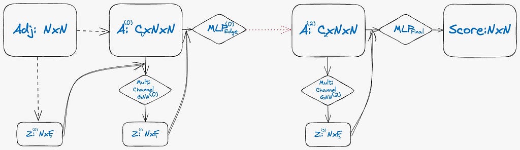
The EDP-GNN layer functions by processing an input consisting of a C-channel adjacency matrix accompanied by node features and outputs an updated C’-channel adjacency matrix also with node features.
The computation of node features is conducted using the Multi-Channel GNN layer. Subsequently, a new C’-channel adjacency matrix is generated. This process involves utilizing the newly computed node features in conjunction with the original C-channel adjacency matrix. The method integrates these elements using concatenation and a Multilayer Perceptron (MLP) network. This approach underlines the layer’s efficiency in transforming and updating the graph structure.
In this approach to modeling undirected graphs, it’s essential to maintain the symmetry of the predicted adjacency matrix. To achieve this, we sum the predicted matrix with its transposed version. This process ensures that the final adjacency matrix accurately reflects the undirected nature of the graph. For a more comprehensive understanding of this transformation, detailed formulas are provided below.

The final network is represented by three layers as we can see on the image. Before being inputted into our EDP-GNN model, graphs undergo preprocessing. This involves using two-channel adjacency matrices: one channel for the original adjacency matrix and the other for its negated counterpart, with all entries inverted. Additionally, we initialize node features based on the weighted degrees of the nodes. This process ensures the graphs are optimally formatted for processing by the EDP-GNN model.
Specifically, if we have node features X from the data, then the initial value for each node is as follows.

A final point to note is that the dimensions of the inputs and outputs in our network are identical. This aspect is crucial because the network is designed to model the score function. Maintaining consistent dimensions ensures that the network accurately represents and processes the score function, which is vital for the model’s effectiveness.
As previously mentioned, it’s necessary to condition each layer of our network on various noise levels. We achieve this noise conditioning by introducing a few learnable parameters, specifically by adding gains and biases. A conditional Multilayer Perceptron (MLP) layer is represented as:

Where α and β are learnable parameters for each noise level σ.
In this post, we have explored the training and sampling process of a score-based graph generation method. This method leverages Graph Neural Networks (GNNs) to preserve the critical inductive bias of permutation invariance in the generated graphs. Furthermore, we demonstrated how the EDP-GNN network can be implemented using PyG utilities. If you want to delve deeper into the technical details, we encourage you to read the original paper available at https://arxiv.org/abs/2003.00638. Thank you for joining us on this learning journey!
[1] C. Niu, Y. Song, J. Song, S. Zhao, A. Grover, and S. Ermon,
Permutation Invariant Graph Generation via Score-Based Generative Modeling, (2020), AISTATS 2020
[2] Song, Y. and Ermon, S. (2019). Generative modeling by estimating gradients of the data distribution. arXiv preprint arXiv:1907.05600
[3] Xu, K., Hu, W., Leskovec, J., and Jegelka, S. (2018a). How powerful are graph neural networks? arXiv preprint arXiv:1810.00826
[4] Jonathan Ho, Ajay Jain, Pieter Abbeel. Diffusion Probabilistic Models https://arxiv.org/abs/2006.11239
[5] Yang Song. Diffusion and Score-Based Generative Models YouTube video. https://youtu.be/wMmqCMwuM2Q?si=64WID5_82zywM6_C
<hr><p>PyG Implementation of EDP-GNN: Generation via Score-Based Generative Modeling was originally published in Stanford CS224W: Machine Learning with Graphs on Medium, where people are continuing the conversation by highlighting and responding to this story.</p>