DL Under the Hood: Tensors, Views, and FLOPs

This post explores what happens under the hood when we create and operate on tensors in PyTorch. From device placement to memory sharing and floating-point operation (FLOP) counts, we’ll see how tensor computations map to real hardware usage and performance.

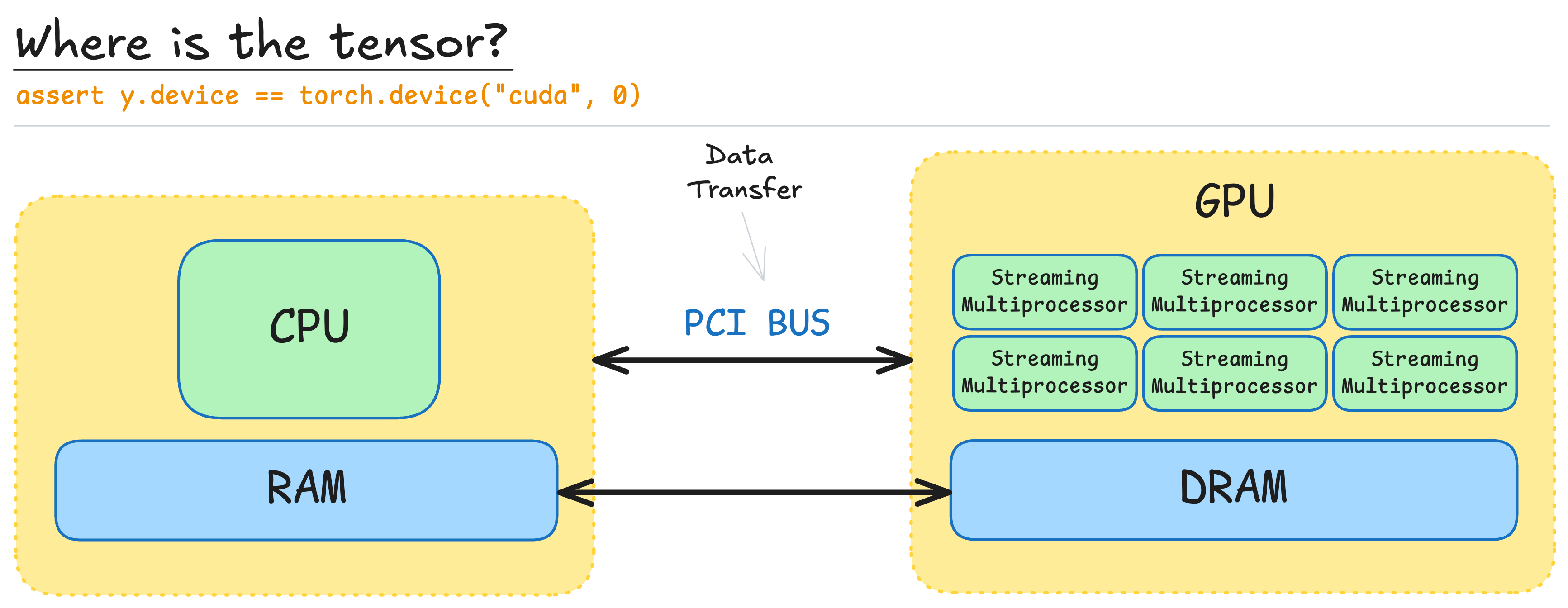
Introduction: Tensors and Memory (CPU vs GPU)

By default, tensors are stored in CPU memory: x=torch.zeros(32, 32).
if GPU is available, we can move tensor there: x.to('cuda:0').
or create it directly on GPU: x=torch.zeros(32, 32, device = 'cuda:0').

Notes:

• To leverage GPU acceleration, we must ensure tensors are on the GPU. This is key to unlocking its massive parallelism.
• Always know where your tensor lives: assert x.device == torch.device('cpu').

Useful PyTorch Utilities:

• torch.cuda.is_available() - check if GPU is available, returns True or False.
• torch.cuda.get_device_properties(i) - inspect GPU “i” specs, returns information about GPU number “i”.
• torch.cuda.memory_allocated() - returns allocated memory, great for debugging memory used by tensors.
• Check if two tensors share the same underlying memory:

  def same_storage(x: torch.Tensor, y: torch.Tensor): -> bool
    x.untyped_storage().data_ptr() == y.untyped_storage().data_ptr()
  

Tensor Storage and Views

Tensors in PyTorch are pointers into allocated memory. Each tensor stores metadata that describes how to access any specific element in that memory block.

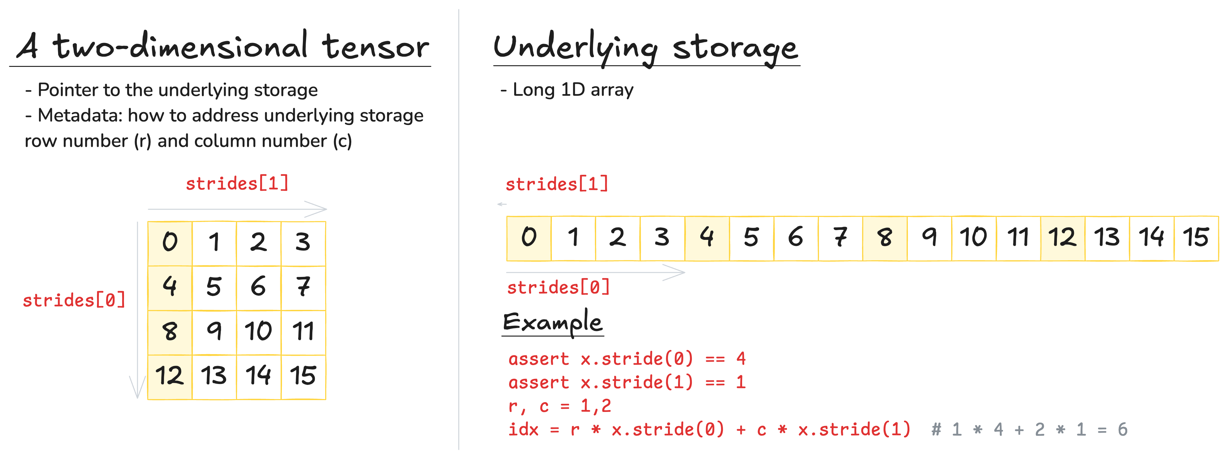
This is important because multiple tensors can share the same underlying storage — even if they represent different shapes or slices. These are called views, and they do not allocate new memory.

Examples:

• slicing

  y = x[0]
  assert same_storage(y, x[0])
  

• taking a view

  x = torch.randn(3,2)
  y = x.view(2,3)
  assert same_storage(y, x)
  

• transposing

  x = torch.randn(3,2)
  y = x.transpose(0,1)
  assert same_storage(y, x)
  

If we modify a tensor through one of its views, the change will be visible through all other — since they share the same memory.

Notes:

• Some views are non-contiguous entries. It means further views are not possible.
  Contiguous means when we iterate over the tensor, we’re reading memory sequentially, not jumping or skipping around.
  Some operations (like .view()) require the tensor to be contiguous. If it’s not, you can fix that using .contiguous(), which copies the data into a contiguous layout.

• Elementwise operations create new tensors: .triu() (helps create a causal attention mask), .pow(2), .sqrt(), .sqr(), etc.

Matrix Multiplication in PyTorch

From linear algebra we remember that matrix multiplication requires the inner dimensions match — the number of columns in the first matrix must be equal the number of rows in the second.

x = torch.ones(16, 32)
w = torch.ones(32, 2)
y = x @ w
assert y.size() == torch.Size([16,2])

In deep learning, we often perform the same operation across a batch of inputs, and for token sequences in NLP:

B, L = 128, 1024
x = torch.ones(B, L, 16, 32)
w = torch.ones(32, 2)
y = x @ w
assert y.size() == torch.Size([B, L, 16,2])

Named Dimensions and Einstein Notation

Traditional PyTorch code often relies on positional indexing, which becomes error-prone when tensors have many dimensions:

B, S, H = 2, 2, 3
x = torch.ones(B, H, S) # batch, sequence, hidden
y = torch.ones(B, H, S) # batch, sequence, hidden
z = x @ y.transpose(-2,-1) # batch, sequence, sequence

But what exactly are -2 and -1? We have to mentally track the meaning of each axis — and that’s fragile.

Proposal: Use named dimensions instead of relying on raw indices. This is where jaxtyping and einops shine:

• Classic style: x = torch.randn(2, 2, 1, 3) # batch seq heads hidden
• Named style: x: Float[torch.Tensor, "batch seq heads hidden"] = torch.randn(2, 2, 1, 3)

Note: We are just documenting, not enforcing. Enforcement is possible, but requires raising check explicitly.

Einstein Summation with einsum
Einstein notation (via einops.einsum) extends matrix multiplication with intuitive dimension bookkeeping. We specify input dims, and what dims remain — everything else is summed over.

• Before
  z = x @ y.transpose(-2, -1)
• After
  z = einsum(x, y, "batch seq1 hidden, batch seq2 hidden -> batch, seq1, seq2")
• Moregenerally, over multiple dimensions
  z = einsum(x, y, "... seq1 hidden, ... seq2 hidden -> ... seq1, seq2")

Other beneficial Einsum Patterns:

• Reduce (e.g. sum over hidden dim): y = reduce(x, "... hidden -> ...", "sum")
• Rearrange (e.g. split/merge heads): x = rearrange(x, "... (heads hidden1) -> ... heads hidden1", heads = 2)
  This replaces the need for view, permute, and reshape — with explicit, readable transformations.

Notes:

• jaxtyping tutorial
• einops tutorial

Measuring Compute: FLOPs and Performance

Definition: A floating point operation (FLOP) is a basic aithmetic operation like addition (a + b) or multiplication (a * b).
Notes: In these notes (and CS336 class), we distinguish:

• FLOPs: total number of floating point operations.
• FLOP/s: floating point operations per second (speed of hardware).

Useful numbers:

• Training GPT-3 (2020) took 3.14e23 FLOPs
• Training GPT-4 (2023) took (rumoured) 2e25 FLOPs (~64x GPT-3)
• US executive order (revoked in 2025): any foundation model trained with 1e26 FLOPs must be reported to the government
• A100 has a peak performance of 312e12 FLOP/s (312 teraFLOP/s); performance for fp32
• H100 has a peak performance of 1979e12 FLOP/s with sparsity, ~50% - -without; performance for fp16 Tensor cores
• RTX5090 is harder to evaluate due to lack of official reports. But following community publications, we can assume that a peak performance for fp16 Tensor cores is higher than 104e12 FLOP/s and lower than 1676e12

Note: Actual performance depends on data types used (e.g., float32 vs bfloat16) and workload structure.
See NVIDIA spec sheets for precise values.
Example Calculation: To train GPT-4 model it is required 2e25 / (1979e12 * 0.5) / (60 * 60 * 24) ~ 2.34e5 H100 days.

Matrix Multiplication: FLOPs Count
Let’s recall how matrix multiplication works:

In general, multiplying a matrix X of shape $B \times D$ with W of shape $D \times K$, produces Y of shape $B \times K$: $y_{ij} = \sum_{k=0}^{D-1} x_{ik} w_{kj}$.

Each element requires

• $D$ multiplications.
• $D-1$ summation (or $D$ summations if we consider creating Y in advance filled with zeros).

Considering that we have $B \times K$ elements, the actual number of flops: 2xBxDxK FLOPs.

Common FLOPs estimates:

• Elemenwise operation on $m \times n$ matrix: O(mn) FLOPs
• Addition of two $m \times n$ matrices: m x n FLOPs
• In generaal, matrix multiplication is by far the most expensive operation in Deep Learning (for large enough matrices). And it is for what GPUs are designed and optimized (large enough matrices).

Interpretation:

• B is the number of data pointes
• (DK) is the number of parameters
• FLOPs for forward pass is ~2 (# tokens) (# parameters) This generalizes for Transformers as well.

Benchmarking Actual FLOPs

To measure actual FLOP/s (wall-clock time), we can time the matrix multiplication and compare against theoretical FLOP/s.

def time_matmul(a: torch.Tensor, b: torch.Tensor) -> float:
    """Returns the number of seconds required to perform 'a @ b'."""

    # Wait until previous CUDA threads are done
    if  torch.cuda.is_available():
        corc.cuda.synchronize()

    def run():
        # performs the operation
        a @ b

        # Wait until previous CUDA threads are done
        if  torch.cuda.is_available():
            torch.cuda.synchronize()

    # Time the operation times
    num_trials = 5
    total_time = timeit.timeit(run, number = num_trials)

    return total_time / num_trials

actual_time = time_matmul(x, w)
actual_flop_per_sec = actual_num_flops / actual_time

Each GPU has official FLOPs specs that report the peak performance:

• A100 [spec]
• H100 [spec]
• RTX5090 [spec; blog1; blog2; blog3]

Model FLOPs utilization (MFU)

Definition: It shows how well you squeeze hardware, it is calculated as \(\frac{\text{actual FLOP/s}}{\text{promised FLOP/s}}\) (ignore communication and overhead).
Note: Usually

• if MFU $\geq 0.5$, it is considered to be very good utilization.
• if MFU $\leq 0.05$, it is considered to be poor utilization.
• MFU is higher, when matrix multiplications dominate.

Conclusion

• Tensors in PyTorch are pointers to memory — reshaping, slicing, and transposing share storage unless you explicitly copy.
• Always know where your tensors live (CPU/GPU) and whether they’re contiguous, to avoid performance inefficiencies.
• Mat. mul. dominates compute: for two matrices of shapes $M \times N$ and $N \times P$, the FLOPs = $2 \times M \times N \times P$.
• FLOP/s depend on hardware (H100 > A100) and data type (bfloat16 > float32).
• Model FLOPs utilization (MFU) measures how efficiently your model uses hardware: \(\text{MFU} = \frac{\text{actual FLOPs}}{\text{theoretical peak FLOPs}}\).