LLM From Scratch: Building TinyGPT that works
In this post I cover the structure and implementation of a minimal Transformer-based LLM - along with practical variants, implementation code, and common pitfalls. Specifically, I’ll:
- Break down the minimal Transformer components.
- Highlight real-world variations for each part.
- Implement each piece from scratch.
- Share results and the key tricks to avoid common pitfalls.
You can view the complete implementation on GitHub.
What does a minimal Transformer-based LLM consist of?
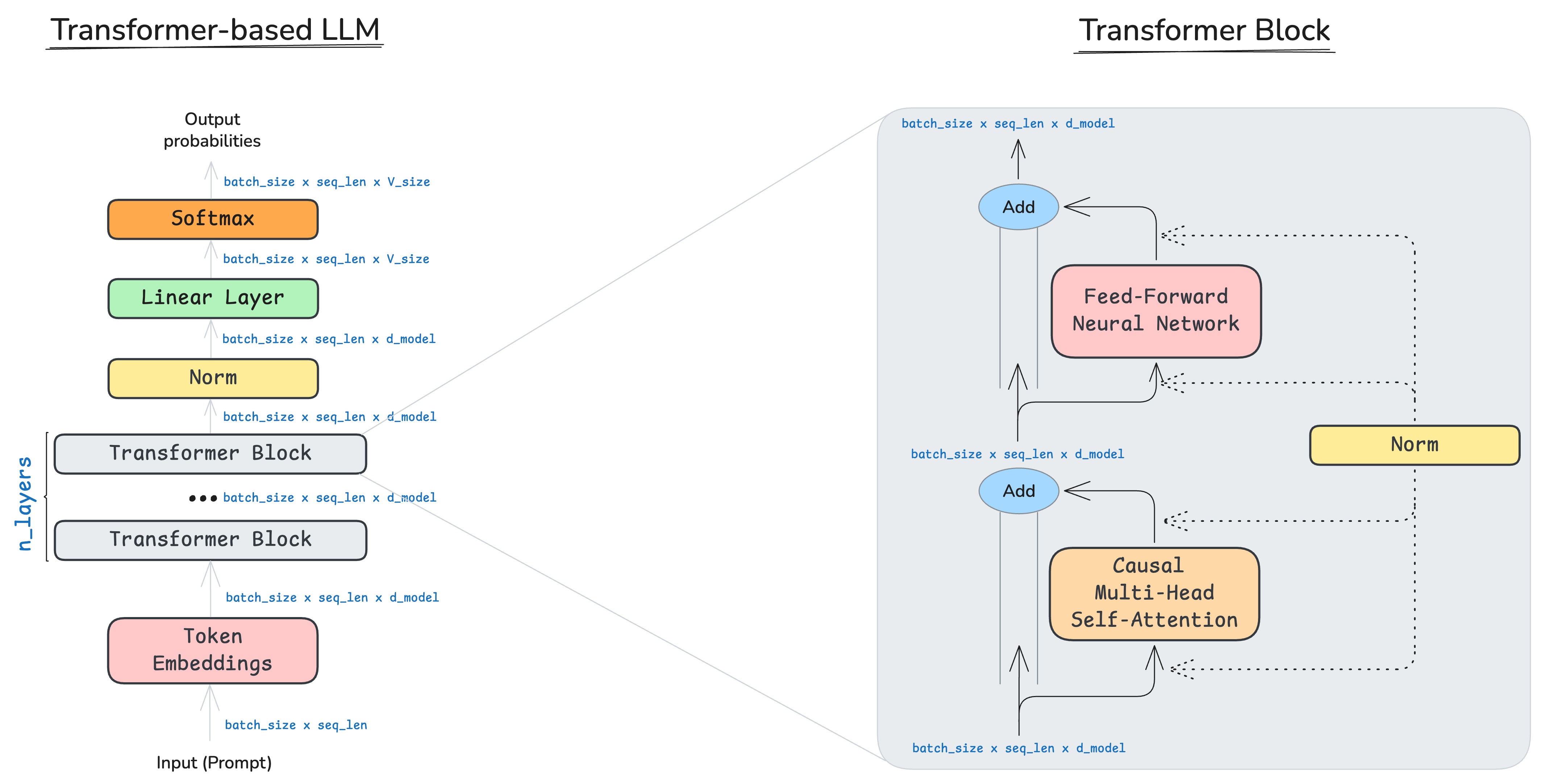
The original Transformer paper (2017) introduced an encoder–decoder architecture for sequence transduction (e.g., machine translation). Decoder-only LLMs keep a stack of Transformer blocks and a final linear head that projects to the vocabulary.
In this post I’ll focus on the minimal components that remain close to the original design and discuss their practical variations. The diagram below shows a decoder-only LLM alongside a single Transformer block.
My implementation of the forward pass:
def forward(self, token_ids, prob: bool = False, tau: float = 1.0):
    x = self.token_embeddings(token_ids)
    x = self.layers(x) # transformer layers
    x = self.ln_final(x)
    logits = self.lm_head(x)
    if not prob:
        return logits
    probs = softmax(logits, dim= -1, tau = tau)
    return probs
Notes:
- Causal masking is applied inside attention for decoder-only models. Encoders are bidirectional and use no causal mask.
- The LM head shares weights with token embeddings in many implementations (weight tying).
With this minimal structure defined, I’ll dive into its most critical component - attention.
Attention (why and what)
Why attention? Before attention, recurrent models dominated, but had issues:
- Bottlenecked memory: hidden state can’t “look back” at specific tokens directly.
- Lack of parallelism: training is sequential across time steps.
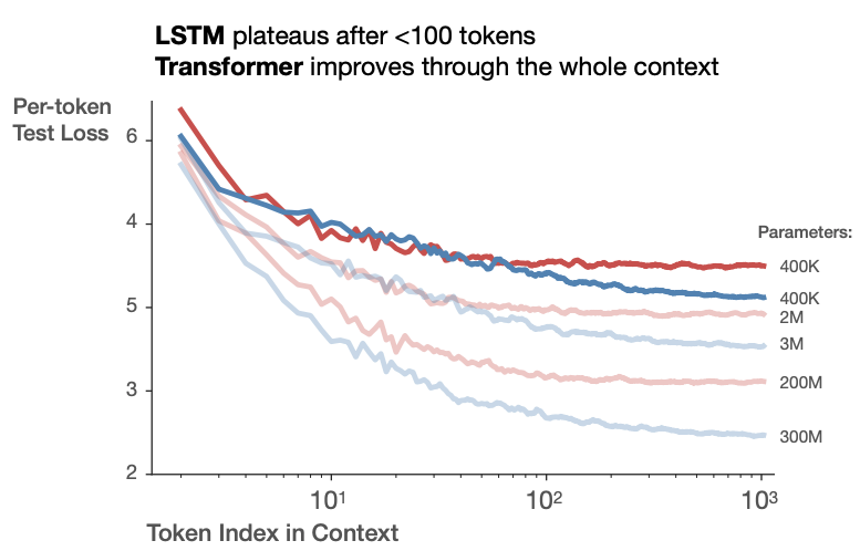
- Long-range dependencies: gradients vanish; longer context helps little in practice (see Kaplan et al., 2020).
- Interpretability: attention’s explicit weights offer a clearer signal than opaque hidden states.
Core idea:
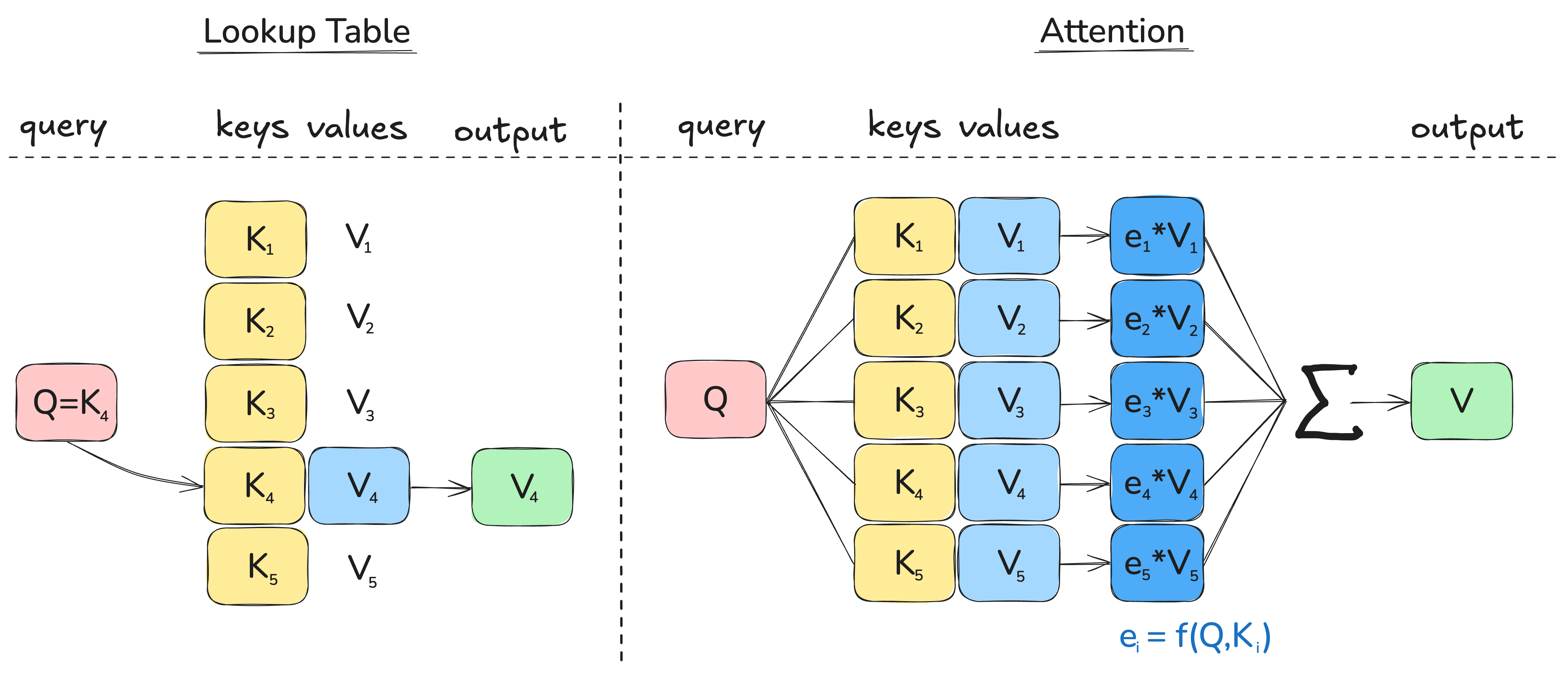
Let each output token attend to all input tokens, weighting their influence by the similarity between query (Q) and key (K). Larger weights mean more focus on those inputs for that output. Q = what this position is looking for, K = what each position offers,
V = the payload to mix. In self-attention, all come from the same sequence via projections: \(Q=xW_Q; K=xW_K; V=xW_V\).
I like the analogy of a soft lookup table - not a single exact match, but a weighted sum over all values. We first compute scores \(s_i\), normalize them with softmax to get weights \(e_i\) so \(\sum_i e_i = 1\), then take \(\sum_i e_i\,V_i\)
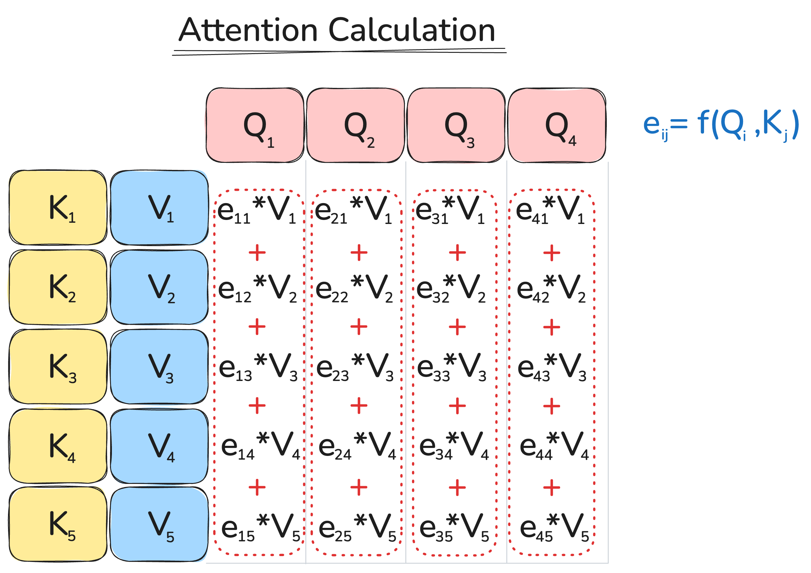
We do this in parallel for all output positions — not just one — which gives the familiar matrix form: \(\text{scores} = QK^T\).
Self-attention is the special case where queries, keys, and values all come from the same sequence. It appears in encoder-only models (bidirectional, no causal mask) and decoder-only models (causal, future masked). Multi-head attention (MHA) computes several such attentions with different learned projections and concatenates the results.
Mostly, attention mechanisms vary in how scores/weights are computed and, to a lesser extent, how queries (Q), keys (K), and values (V) are parameterized.
Attention Variants:
The most common variations of computing attention scores are summarized below.
| Attention Type | Formula | Notes |
|---|---|---|
| Dot Product | $e_i = s^Th_i$ | Naive form, rarely used in practice. No learnable parameters; requires $s$ and $h_i$ to have the same dimensionality. |
| Multiplicative / Bilinear | $e_i = s^TWh_i \in \mathbf{R},\; W \in \mathbf{R}^{d_2 \times d_1}$ | Adds learnable weights and allows different dimensions for $s$ and $h_i$. Introduced by Luong et al., 2015. |
| Reduced-rank Multiplicative | $e_i = s^T(U^TV)h_i = (Us)^T(Vh_i)$ $U \in \mathbf{R}^{k \times d_2},\; V \in \mathbf{R}^{k \times d_1},\; k \ll d_1, d_2$ | Improves computational efficiency by projecting to a smaller dimension $k$. |
| Additive | $e_i = v^T \cdot \tanh(W_1h_i + W_2s) \in \mathbf{R}$ $W_1 \in \mathbf{R}^{d_3 \times d_1},\; W_2 \in \mathbf{R}^{d_3 \times d_2},\; v \in \mathbf{R}^{d_3}$ | Original attention mechanism, introduced by Bahdanau et al., 2014. Computationally heavier than multiplicative attention. |
Pitfalls with “naive” attention (and fixes):
- No notion of order \(\to\) add positional information (Learned PE, RoPE, ALiBi).
- Pure attention layers collapse to weighted averaging \(\to\) stack with a position-wise MLP (FFN) and residuals.
- Information leak from the future \(\to\) Apply causal masks (decoder-only) inside attention: \(\text{scores} = QK^T + M\).
- Dot products scale with dimensionality \(\to\) Divide scores by \(\sqrt{d_k}\): \(\text{scores} = \frac{QK^T}{\sqrt{d_k}} + M\).
- Numerical stability \(\to\) Addressed via proper initialization, normalization, and other techniques (see Stability).
Implementation
Projections to Q/K/V/O
self.d_k, self.d_v = d_model // num_heads, d_model // num_heads

# init projections
self.P_Q = Linear(d_model, num_heads * self.d_k, init_type, clip_w, device = device, dtype=dtype)
self.P_K = Linear(d_model, num_heads * self.d_k, init_type, clip_w, device = device, dtype=dtype)
self.P_V = Linear(d_model, num_heads * self.d_v, init_type, clip_w, device = device, dtype=dtype)
self.P_O = Linear(num_heads * self.d_v, d_model, init_type, clip_w, device = device, dtype=dtype)
Scaled dot-product attention (SDPA).
def scaled_dot_product_attention(Q: torch.Tensor, K: torch.Tensor, V: torch.Tensor, mask: torch.Tensor | None):
    """
    Q, K:  (batch_size, ..., seq_len, d_k)
    V:  (batch_size, ..., seq_len, d_v)
    """
    d_k = K.shape[-1]
    # seq_len is the same for both Q and K, but I distinguish the ordering
    scores = einsum(Q, K, "... seq_len_q d_k, ... seq_len_k d_k -> ... seq_len_q seq_len_k")
    scores = scores.clamp(min = -80, max=80.0)
    if mask is not None:
        scores = scores.masked_fill(~mask, float('-inf'))
    weights = softmax(scores / (d_k ** 0.5), dim = -1)
    att = einsum(weights, V, "... seq_len seq_len2, ... seq_len2 d_v -> ... seq_len d_v")
    return att
It’s worth mentioning that earlier I rearranged dimensions to prepare for multi-head attention, apply RoPE (if necessary), and finally (after applying MHA) project the combined outputs:
def forward(self, x: torch.Tensor, is_masked: bool = True, with_rope = True, token_positions = None):
    # project x to get queries, keys and values
    Q = self.P_Q(x)
    Q = rearrange(Q, "... seq_len (h d_k) -> ... h seq_len d_k", h = self.num_heads)
    K = self.P_K(x)
    K = rearrange(K, "... seq_len (h d_k) -> ... h seq_len d_k", h = self.num_heads)
    V = self.P_V(x)
    V = rearrange(V, "...  seq_len (h d_v) -> ... h seq_len d_v", h = self.num_heads)
    # apply RoPE
    if with_rope and self.rope is not None:
        Q = self.rope(Q)
        K = self.rope(K)
    # create mask
    if is_masked:
        mask = ~torch.triu(torch.full((Q.shape[-2], K.shape[-2]), True, device = self.device), diagonal=1)
    else:
        mask = None
    # calculate scaled attention
    scaled_mh_att = scaled_dot_product_attention(Q, K, V, mask)
    scaled_mh_att = rearrange(scaled_mh_att, "... h seq_len d_v -> ... seq_len (h d_v)")
    # project on output
    O = self.P_O(scaled_mh_att) # O = einsum(scaled_mh_att, self.P_O, "... seq_len hd_v, d hd_v -> ... seq_len d")
    return O
Positional Information
As I mentioned earlier, the “naive” version of attention has no notion of order - its output is permutation invariant.
In the original “Transformer” paper, the authors introduced sinusoidal position representations:
\[\text{PE}(pos, 2i) = \sin\!\left(\frac{pos}{10000^{2i/d}}\right), \quad \text{PE}(pos, 2i+1) = \cos\!\left(\frac{pos}{10000^{2i/d}}\right)\]These fixed vectors were added to token embeddings before feeding them into the encoder or decoder stack. This approach has no learnable parameters and was motivated by the idea that the periodic functions would enable extrapolation to longer sequences, though in practice this effect was limited.
A later and widely used alternative is learned positional embeddings, where position vectors are learned jointly with the model. Adopted by BERT, GPT-2, and many successors, these embeddings are added to token vectors in the same way as before:
x = token_embed(input_ids) + position_embed(pos_ids)
Finally, most modern LLMs (e.g., LLaMA, GPT-NeoX) use Rotary Positional Embeddings (RoPE), which encode relative position information by rotating the query and key vectors. Rotation is applied in pairs of coordinates, each using a different frequencies:
RoPE operates inside the attention mechanism, rotating the query and key vectors before computing attention scores.
Implementation
Below is a minimal PyTorch implementation of RoPE used in modern LLMs (e.g., LLaMA, GPT-NeoX):
class RoPE(nn.Module):
    def __init__(self, theta: float, d_k: int, max_seq_len: int, device: torch.device | None = None, dtype: torch.dtype | None = None):
        super().__init__()
        assert d_k % 2 ==0
        self.d_k = d_k
        # rotate over even indices
        position = torch.arange(max_seq_len, dtype=dtype, device=device)
        inv_freq = 1.0 / (theta ** (torch.arange(0, d_k, 2, dtype = dtype, device = device) / d_k))
        emb = einsum(position, inv_freq, "max_seq_len, half_d_k -> max_seq_len half_d_k")
        # register sin and cos
        self.register_buffer("sin", torch.sin(emb), persistent=False)
        self.register_buffer("cos", torch.cos(emb), persistent=False)

    def forward(self, x: torch.Tensor, token_positions: torch.Tensor | None = None) -> torch.Tensor:
        assert x.shape[-1] == self.d_k
        # choose right positions
        if token_positions is None:
            token_positions = torch.arange(x.shape[-2])
            token_positions = token_positions.to(self.sin.device)
        sin = self.sin[token_positions]
        cos = self.cos[token_positions]
        # split x into even and odd dimensions
        x1 = x[..., 0::2]
        x2 = x[..., 1::2]
        # apply rotations (it will broadcast automatically since last 2 dims match)
        rot_x1 = x1 * cos - x2 * sin
        rot_x2 = x1 * sin + x2 * cos
        # calculate output
        x_out = torch.empty_like(x) # torch.zeros_like(x) is slower in theory
        x_out[..., 0::2] = rot_x1
        x_out[..., 1::2] = rot_x2
        return x_out # Rotated queries/keys with position encoding applied
Why Feed-Forward (MLP) Block?
The Feed-Forward Network (FFN) sits on top of attention and introduces a non-linearity for each token’s representation. We need it to stack multiple layers and learn complex transformations — just like ReLU or GeLU do in CNNs for computer vision.
The often-repeated phrase “applied to each token output separately” doesn’t imply a special operation. It means that the same linear layers and activations are broadcast across all tokens — in dense FFNs matrix multiplication naturally does this in parallel. In Mixture-of-Experts (MoE) architectures, each token may be routed to a different expert, so while tokens are still processed independently, the applied parameters can differ per token.
Applications of FFNs in Transformers differ mainly by three aspects:
- FFN structure: Gated vs Non-gated.
- Choice of non-linearity: ReLU, GELU, Swish, Squared ReLU
- Placement relative to Attention: sequential vs parallel.
Gated vs Non-Gated
In the non-gated setup, we apply the classic sequence: linear layer, followed by a non-linearity, and then another linear layer. The gated FFN adds one more linear projection that transforms the input and applies an element-wise multiplication between this projection and the nonlinear output. As of today, most architectures use gated activations, but it is not a game changer. The illustration below compares both designs.
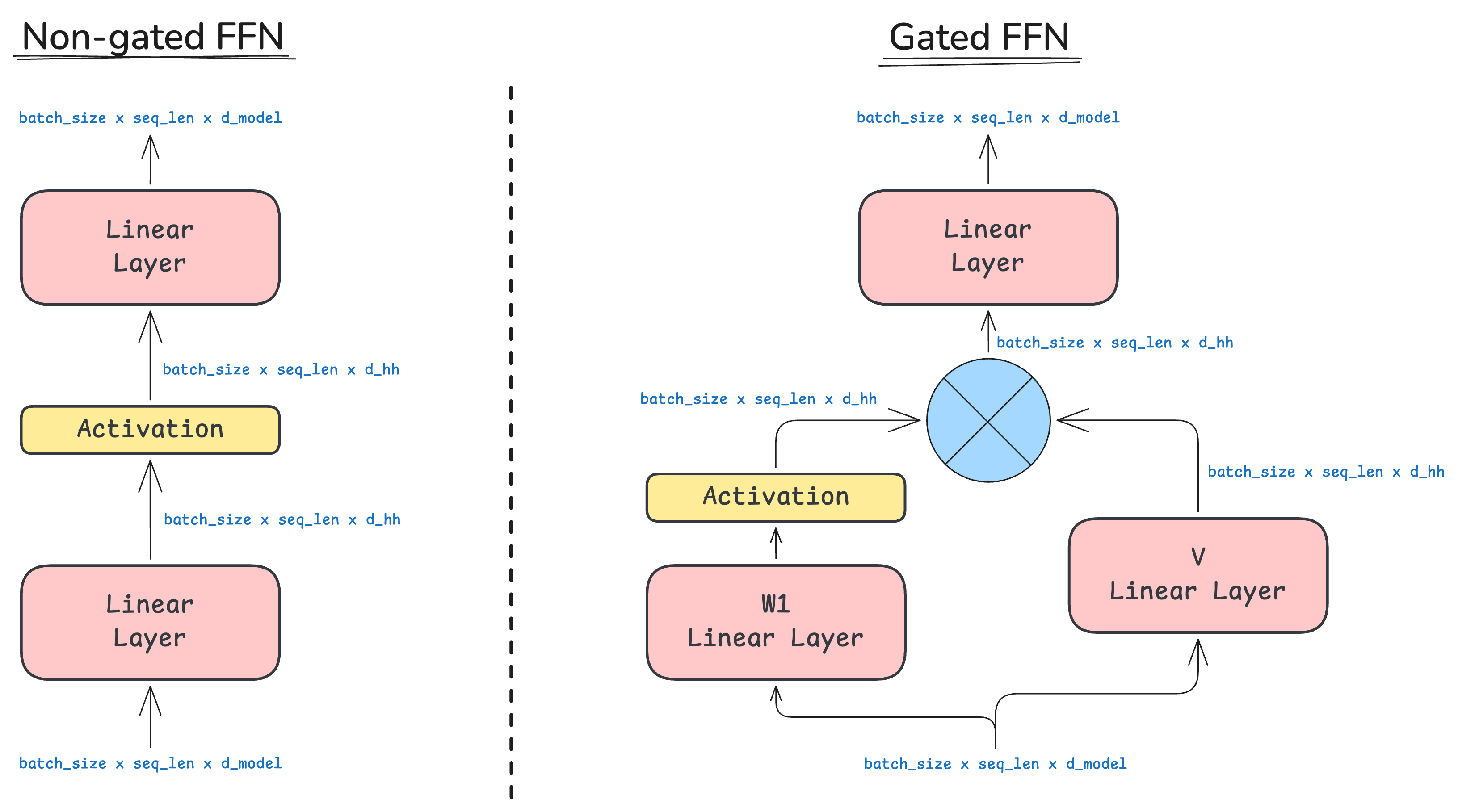
In most modern LLMs, non-gated FFNs use \(d_{\text{hh}} \approx 4 \times d_{\text{model}}\), while gated version use \(d_{\text{hh}} \approx 8/3 \times d_{\text{model}}\). This keeps parameter count roughly constant between designs. There are exceptions - T5 (Raffel et al, 2020) uses a much larger ratio of 64x.
Choice of non-linearity
Different architectures use different activation functions inside the FFN. Common choices:
| Activation | Formula | Notes |
|---|---|---|
| ReLU | $\max(0, x)$ | Simple and fast; used in the original Transformer. |
| GELU | $x \cdot \Phi(x)$ | Smooth probabilistic version of ReLU; gated version used in Phi-3, Gemma-2, Gemma-3. |
| Swish | $x \cdot \sigma(x)$ | Smooth and continuously differentiable; gated version used in LLaMA 1/2/3, PaLM, Mistral. |
| Squared ReLU | $(\max(0, x))^2$ | Improves expressivity; efficient for sparse LLMs (Zhang et al., 2024). |
Implementations are below.
class ReLU(nn.Module):
    def forward(self, x):
        return torch.where(x < 0, torch.zeros_like(x), x)

class LeakyReLU(nn.Module):
    def __init__(self, alpha: float = 0.01):
        super().__init__()
        self.alpha = alpha
    def forward(self, x):
        return torch.where(x < 0, self.alpha * x, x)

class SqReLU(nn.Module):
    def forward(self, x):
        return torch.where(x < 0, torch.zeros_like(x), x ** 2)

class SiLU(nn.Module):
    def forward(self, x):
        return x * torch.sigmoid(x)

class GELU(nn.Module):
    def forward(self, x):
        return 0.5 * x * (1 + torch.tanh(math.sqrt(2/ math.pi) * (x + 0.044715 * x ** 3)))
Parallel vs Sequential
To introduce non-linearity, the common design applies the FFN after attention (sequential):
\[\text{Output} = \text{FFN}(\text{Attention}(x))\]Some architectures instead place it in parallel, summing both outputs before normalization or residual addition:
\[\text{Output} = \text{Attention}(x) + \text{FFN}(x)\]Parallel placement can improve gradient flow and stability in very deep models, and it is also more parallelizable.
Stability: Norms, Residuals, and more
Training large language models is challenging, and instability can appear in several ways. Common symptoms and their potential causes are summarized below:
| Symptom | Potential Reason |
|---|---|
| Loss becomes $\text{NaN}$ | Exploding gradients or numerical overflow. |
| Loss does not decrease or decreases too slowly | Poor initialization or learning rate too small. |
| Divergence after several epochs | Learning rate too large or instability from mixed precision. |
| Evaluation much worse than Training | Incorrect normalization or dropout handling. |
The first issue - loss becoming $\text{NaN}$ - is by far the most common. What typically causes it?
- Exponentials or other functions where \(\|f(x)\| \gg \|x\|\).
- Division by (or near) zero.
Normalization
Early Transformers and major LLMs - GPT 1/2/3, OPT, BLOOM - used LayerNorm, which normalizes both mean and variance across the feature dimension $d_{\text{model}}$:
\[\text{LayerNorm:}\quad y = \frac{x - \mathbf{E}[x]}{\sqrt{\text{Var}[x] +\epsilon}}\cdot \gamma +\beta\]Recent models s.a. LLaMA-1/2/3, PaLM, and T5 switched to RMSNorm, which normalizes only by the root-mean-square value:
\[\text{RMSNorm:}\quad y = \frac{x}{\sqrt{\mathbf{E}[x^2]} + \epsilon}\cdot \gamma\]RMSNorm is slightly faster and performs on par with LayerNorm, making it the default choice in most modern architectures.
Where is it placed?
In most models, normalization is applied to the inputs of each block (attention and MLP). However, there are some notable exceptions:
- OLMo2 (Walsh et al.) applies normalization to the outputs of blocks.
- Gemma 2 (DeepMind, 2024) applies normalization to both inputs and outputs.
Some architectures go even further, applying normalization:
- to Q and K projections inside attention (e.g., Qwen-3, LLaMA-3, DeepSeek-V2)
- to the inputs of softmax operations to improve numerical stability.
Residual Connections
Residual connections address the problem of vanishing gradients in deep networks. They allow gradients to flow directly through identity paths, making optimization stable even with hundreds of layers. Since their introduction in ResNets (He et al., 2015) and later RNN-based architectures (Kim et al, 2017), residuals have become a standard component of nearly all LLM designs.
Variance Scaling
In the original Transformer paper (Vaswani, 2017), the authors introduced scaled dot-product attention, dividing $QK^T$ by $\sqrt{d}$ (or by $d_k=\sqrt{d/h}$ for multi-head attention). The goal was to prevent large dot-product magnitudes caused by high dimensionality $d_k$, which could push softmax into regions with vanishing gradients.
The same idea - variance scaling - can help elsewhere in the model. For instance, when using weight tying, I observed overflow in the output logits. Scaling them by $1/\sqrt{d_{\text{model}}}$ stabilized training:
if self.wt:
    logits /= self.d_model ** 0.5
This trick can be applied after any “ready-to-explode” layer to keep activations numerically stable.
Initialization
Proper weight initialization helps prevent overflow, vanishing, and exploding gradients early in training. For linear layers, the most common schemes are:
| Initialization | Formula | Pros | Cons |
|---|---|---|---|
| Xavier (Glorot) | $$\text{std} = \sqrt{\frac{2}{n_\text{in} + n_\text{out}}}$$ | Balances variance between input/output; good for symmetric activations like tanh, sigmoid. | Can underperform with ReLU-like activations. |
| Kaiming (He) | $$\text{std} = \sqrt{\frac{2}{n_\text{in}}}$$ | Designed for ReLU-family activations; prevents early layer saturation. | Can produce larger initial variance for very deep nets. |
| LeCun | $$\text{std} = \sqrt{\frac{1}{n_\text{in}}}$$ | Suited for SELU / Swish or scaled activations. | Less common in LLMs. |
| Squared Kaiming | $$\text{std} = \frac{2}{n_\text{in} + n_\text{out}}$$ | Works well in LLMs without weight tying. | Can be too aggressive; niche use. |
Typical embedding initialization uses mean $0$ and standard deviation between $0.02$ and $1.0$. However, the optimal scale depends on context — for example, when using weight tying, a smaller standard deviation ($\approx 0.02$) prevents overflow in logits.
My implementation is below:
# create new weight
if init_type == "xavier":
    std = (2 / (in_features + out_features)) ** 0.5
elif init_type == "sq_xavier": # surprisingly, it worked
    std = 2 / (in_features + out_features)
elif init_type == "kaiming":
    std = (2 / in_features) ** 0.5
elif init_type == "lecun":
    std = (1 / in_features) ** 0.5

data = torch.empty(out_features, in_features, dtype=dtype, device=device)
if clip_w is not None:
    nn.init.trunc_normal_(data, mean=0.0, std=std, a=-clip_w, b=clip_w)
else:
    nn.init.normal_(data, mean=0.0, std=std)
Z-loss
To understand this trick, let’s first recall the softmax formulation:
\[P(x) = \frac{e^{U_r(x)}}{Z(x)},\quad Z(x) = \sum_{r'=1}^{|V|} e^{U_{r'}(x)}\]One common source of numerical instability is an exploding partition function \(Z\). To mitigate this, the Z-loss adds a penalty term that encourages \(Z\) to be close to \(1\):
\[L = \sum_i \big[ -\log P(x_i) + \alpha \, (\log Z(x_i))^2 \big]\]This helps prevent excessively large logits and stabilizes mixed-precision training. The idea was first introduced in large-scale LLM training by PaLM (Chowdhery et al, 2022), where a typical value for \(\alpha\) is \(10^{-4}\).
Gradient Clipping
Another standard method to control exploding gradients is gradient clipping. Before each optimizer step, gradients are rescaled if their norm exceeds a chosen threshold. If \(\|g\|_2 > \tau,\quad g \leftarrow g \cdot \frac{\tau}{\|g\|_2}\). Typical clipping thresholds are in the range \(0.5–5.0\), with \(1.0\) being commonly a default value. This keeps the optimizer updates bounded and prevents \(\text{NaNs}\) in mixed-precision training. Gradient clipping is a simple and effective safeguard against divergence, though it can mask poor initialization or suboptimal learning rate if overused.
Implementation example:
def gradient_clipping(model, max_l2_norm: float, eps: float = 1e-6):
    """
    returns pre-clipping and after-clipping gradient value for logging
    """
    assert max_l2_norm > 0, f"Max L2 norm should be positive but it is {max_l2_norm}."
    # get global norm
    sum_sq = None
    for param in model.parameters():
        g = param.grad
        if g is not None:
            if sum_sq is None:
                sum_sq = torch.zeros(1, device = g.device)
            sum_sq += g.detach().float().pow(2).sum()
    # check if no gradients or current norm is too large
    if sum_sq is None:
        return None, None
    global_l2_norm = sum_sq.sqrt()
    if global_l2_norm <= max_l2_norm:
        return global_l2_norm.item(), global_l2_norm.item()
    # update gradients
    scale = max_l2_norm / (global_l2_norm + eps)
    grad_device = global_l2_norm.device
    sum_sq = torch.zeros(1, device = grad_device)
    with torch.no_grad():
        for param in model.parameters():
            if param.grad is not None:
                param.grad.mul_(scale.to(param.grad.dtype))
                sum_sq += param.grad.detach().float().pow(2).sum()
    return global_l2_norm.item(), sum_sq.sqrt().item()
I logged the global pre-clip L2 gradient norm in Weights & Biases. The plots show occasional spikes above the \(1.0\) threshold; clipping at \(1.0\) flattens these excursions and prevents overflow/NaNs in mixed precision. I also track the post-clip norm to confirm it equals \(\min(\lVert g\rVert_2,\ 1.0)\). Screenshot for pre-clip gradient runs with spikes are below.

Learning Rate Warmup and Schedule
A learning rate that’s too large can cause overflow or gradient explosions, while one that’s too small leads to slow convergence. What’s “too large” or “too small” depends on context:
- At the start of training (when weights are random), a large LR often causes divergence.
- Near the end, a smaller LR helps the model settle into a stable minimum.
To handle these dynamics, we use learning rate scheduling with warmup:
- Warmup - gradually increase the LR from a small value to the target LR during the first steps. This prevents large, unstable updates while activations and gradients are still noisy.
- Scheduling (decay) – after warmup, gradually decrease the LR to stabilize optimization near convergence. This helps fine-tune weights rather than overshooting minima.
One of the most common approaches is the cosine scheduler with warmup: \(\text{LR}(t) = \begin{cases} \text{LR}_\max \cdot \frac{t}{N_\text{warmup}}, & t < N_\text{warmup} \\ \text{LR}_\max , & N_\text{warmup} \le t < N_\text{flat} \\ \text{LR}_\min + \text{LR}_\max \cdot \frac{1}{2}\left(1+\cos\frac{\pi (t-N_\text{flat})}{N_\text{cosine}-N_\text{flat}}\right), & N_\text{flat} \le t < N_\text{cosine} \end{cases}\)
My implementation is below:
def cosine_lr_schedule(t: int, lr_max: float, lr_min: float, warmup_iters: int, flat_iters: int, cosine_cycle_iters: int):
    assert warmup_iters >= 0, f"Invalid warmup iterations: {warmup_iters}"
    assert  cosine_cycle_iters > warmup_iters, f"Invalid cosine cycle iterations: {cosine_cycle_iters}"
    # warm up
    if t < warmup_iters:
        return t / warmup_iters * lr_max
    # flat
    if t < flat_iters:
        return lr_max
    # cosine annealing
    if t < cosine_cycle_iters:
        return lr_min + 0.5 * (1 + math.cos((t - flat_iters) / (cosine_cycle_iters - flat_iters) * math.pi)) * (lr_max - lr_min)
    # post annealing
    return lr_min
Weight Decay
Weight decay is traditionally used as a form of regularization, discouraging large weights to reduce overfitting. However, in LLMs the situation is different — we usually train on massive datasets, often with far more tokens than parameters, so classical overfitting is rarely the main concern. So why do we still use weight decay in modern LLM training?
D’Angelo et al., 2023 showed that the primary effect of weight decay in LLMs is not regularization, but rather stabilizing the optimization dynamics. It smooths the loss landscape and improves convergence, particularly during later training phases when smaller learning rates are used. In practice, it may slow early progress but consistently improves stability and final performance.
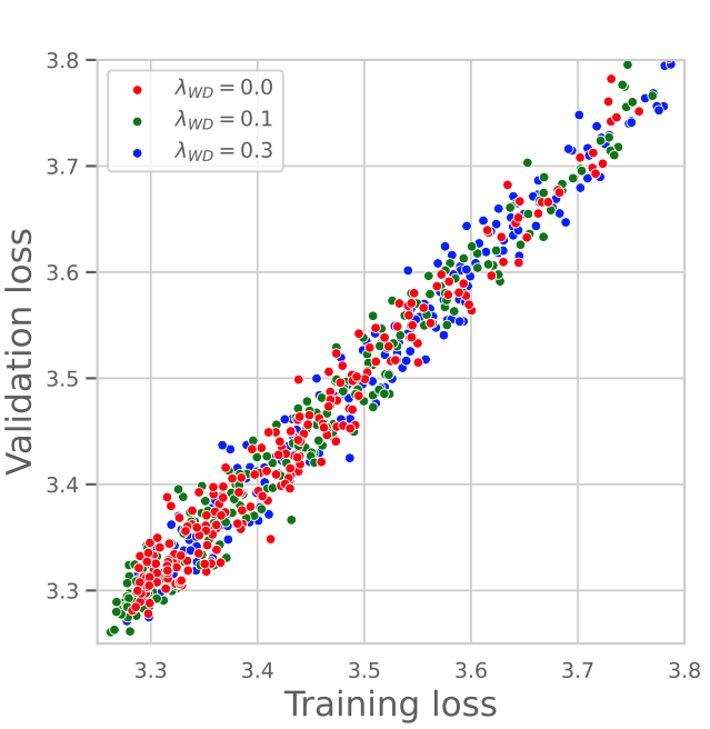
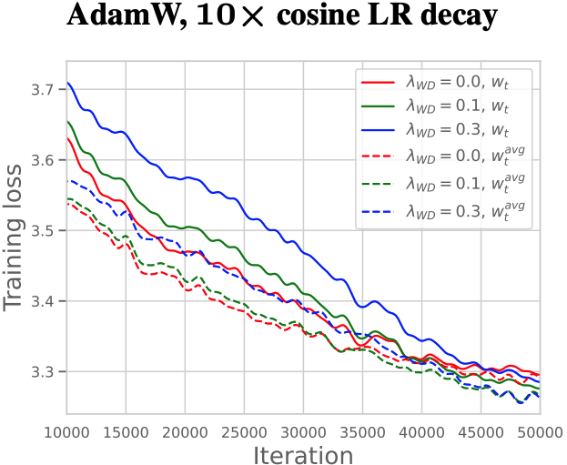
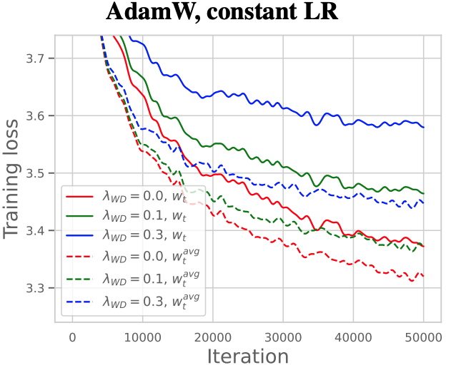
The plots below from their paper illustrate this behavior:
Left: Ratio of validation to training loss (independent of weight decay).
Center: Training loss with $10 \times$ cosine LR schedule.
Right: Training loss with constant LR.
Precision
Modern LLMs are almost universally trained with mixed precision (FP16 or BF16), which can speed up training by $1.5–2 \times$ and reduce memory usage. However, it also introduces potential numerical stability issues that must be handled carefully:
- Overflow risks: pointwise operations where \(\|f(x)\| \gg \|x\|\), e.g. exponents or squared activations.
- Rounding errors: operations that add very small values to large sums, or large reductions like softmax or normalization.
To mitigate these issues, we use loss scaling, FP32 accumulators, and numerically stable implementations (e.g., subtracting the maximum value before softmax).
x_max = x.max(dim=dim, keepdim=True).values # ... x vocab_size -> ... x 1
exps = torch.exp(x - x_max)
For operations prone to overflow, FP16 should be avoided; for those sensitive to rounding errors, higher precision may be required, so BF16 might not be suitable.
Gradient Accumulation
Gradient accumulation allows us to simulate larger batch sizes when GPU memory is limited. Instead of updating weights after every mini-batch, gradients are accumulated across several forward–backward passes, and the optimizer step is taken only after \(N\) accumulation steps.
This approach helps:
- Emulate large-batch training without increasing memory usage.
- Reduce gradient noise and make optimization more stable.
- Trial larger effective batch sizes before scaling to multi-GPU.
Caveats:
- Learning rate scaling: the effective batch size grows with the number of accumulation steps, so the learning rate must be adjusted accordingly — typically following the linear (\(\text{LR} \propto \text{batch size}\)) or the square-root (\(\text{LR} \propto \sqrt{\text{batch size}}\)) scaling. In practice, tuning is still required to find the most stable setting.
- Scheduler steps: learning rate schedulers should advance once per optimizer step, not per micro-step.
A high-level implementation is shown below:
# optimization step
model.train()
for step in loop:
    # zeroing gradients before starting accumulation
    optimizer.zero_grad()

    loss_acc = 0
    # gradient accumulation step
    for i in range(accum_steps):
        tokens_curr, tokens_next = data_loading(...)
        logits = model(tokens_curr)
        loss = loss_fn(logits, tokens_next)

        # average gradient across micro-batches
        (loss / accum_steps).backward()
        loss_acc +=  loss.item() / accum_steps

    # optimizer step
    optimizer.step()
Inference Tricks
To recall, at each decoding step, the LLM predicts a probability distribution over all vocabulary tokens. In this chapter, I briefly cover several inference tricks that improve latency and generation fidelity, each with its own trade-offs.
Top-k sampling
One of the simplest ways to improve generation fidelity is to sample only from the top-k tokens with the highest predicted probabilities, rather than from the entire vocabulary. This ensures the model never selects a token with extremely low confidence.
The small drawback is a slight reduction in diversity, since low-probability tokens are excluded.
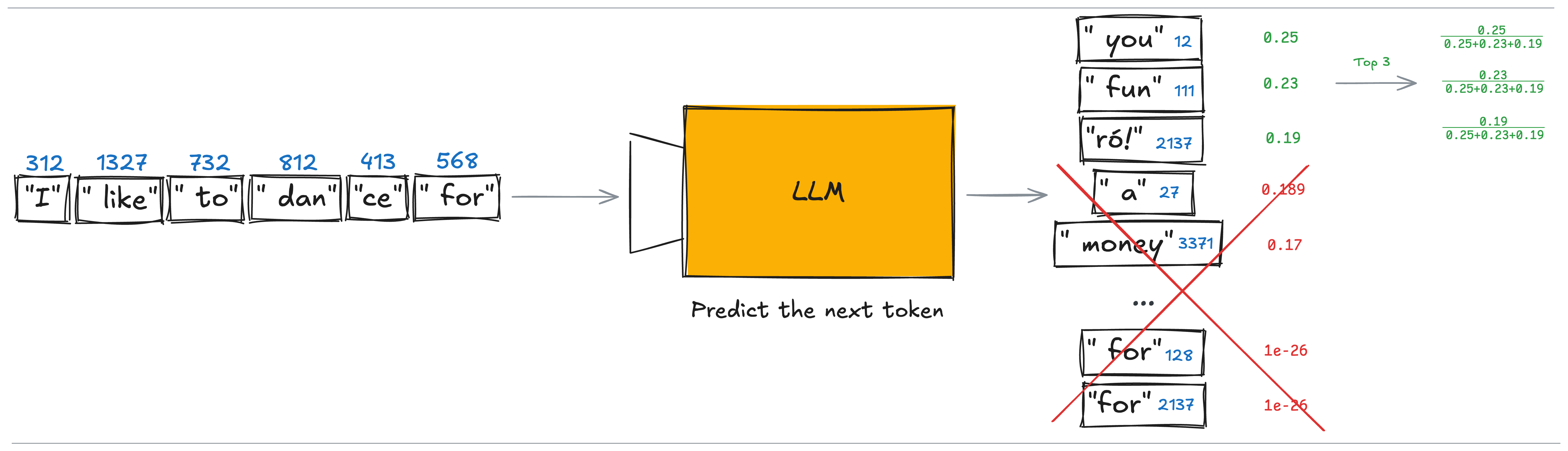
It’s worth noting that both the inputs and outputs of an LLM are token indices. After sampling, the model returns an index that is then decoded back into text using the tokenizer. In the simple example above, one of the top three tokens is chosen - and after decoding, we might get something like:
I like to dance forró!
Note: Forró - a traditional Brazilian dance - happens to be one of my favorites. :)
Temperature in softmax
Temperature $\tau$ is a parameter applied to the logits inside the softmax: $ e^{\text{logit}_i} \to e^{\text{logit}_i \ /\tau}$. It controls the sharpness of the output distribution - lower values ($\tau < 1$) make probabilities sharper, while higher values ($\tau > 1$) make them flatter and increase randomness. The goal is similar to top-k sampling - favoring high-probability tokens while reducing the chance of sampling low-confidence ones.
Why does it work?
Let’s assume that \(\text{logit}_i > \text{logit}_j\), and compare how ratio of their softmax probabilities changes with different values of \(\tau\):
Since \(\tau > 0\) and \(\text{logit}_i > \text{logit}_j\), this ratio is always \(>1\). However, the smaller the value of \(\tau\), the larger the gap between two probabilities - making the distribution sharper.
Conversely, as \(\tau \to +\infty\), we get $\text{softmax}_i \approx \text{softmax}_j$, meaning the model samples from the vocabulary almost uniformly, resulting in random-like generation.
KV Cache
The LLMs discussed in this post are autoregressive - they generate one token at a time, with each new token depending on all previous ones. This process cannot be parallelized across sequence steps.
Let’s look at two consecutive steps of token generation. Specifically, I’ll examine what happens inside the Attention block then generalize the idea to the Feed-Forward Network (FFN). Note that the batch_size dimension doesn’t affect the logic here, since each sequence is processed independently.
I’ll also omit num_heads, as heads are processed in parallel within attention and don’t appear in FFNs.
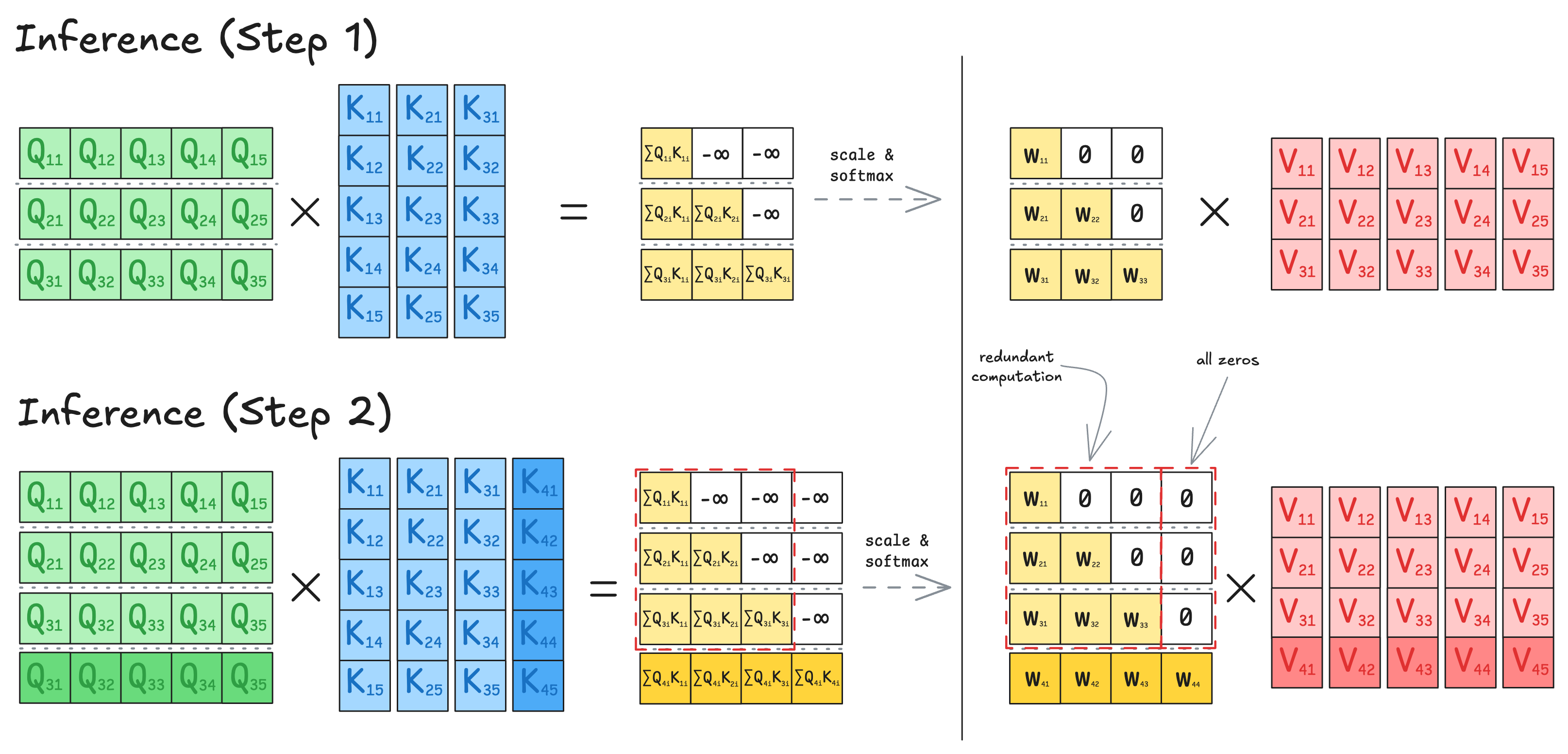
It’s easy to see that at every new step, the model recomputes all previous key and value projections (K, V) - even though they haven’t changed - just to add one new pair of vectors. The solution is the KV Cache: store previously computed $K$ and $V$ projections in memory, and at each step, compute only the new ones. This technique dramatically speeds up inference, but also introduces significant memory overhead.
Later post will cover KV-cache compression and attention variants (MQA, GQA, MLA) that address the memory-speed trade-off.
Notes:
Without a KV cache, the input and output of each Transformer block have dimensions \(\text{(seq_len)} \times d_{\text{model}}\), since all tokens are processed at once. With KV caching, we only process one new token at each step, so the input and output reduce to \(1 \times d_{\text{model}}\).
Unlike attention, FFNs are position-wise: each token is processed independently with shared weights. During incremental decoding you only need to run the FFN on the new token (shape \(1 \times d_{\text{model}}\)); there’s nothing to cache from previous steps.
Common Configurations to Start From
Large language models involve many hyperparameters, yet most of them remain relatively consistent across architectures. To give a clearer high-level overview — and to help dive into LLM design faster — I’ve summarized the key configuration patterns. Models are grouped into Small, Medium, and Large, and each group includes both Factual (architectural) and Numeric details.
Small Models
Factual configuration
| Name | Lab | Year | Params(B) | Norm | Layer Type | Pre/Post-Norm | Positional Embedding | Activation |
|---|---|---|---|---|---|---|---|---|
| Original Transformer | 2017 | 0.213 | LayerNorm | Sequential | Post-Norm | Sinusoidal | ReLU | |
| BERT-Large | 2018 | 0.34 | LayerNorm | Sequential | Post-Norm | Absolute (LE) | GELU | |
| T5-3B | 2019 | 2.8 | RMSNorm | Sequential | Pre-Norm | Absolute (LS) | ReLU | |
| GPT-J-6B | EleutherAI | 2021 | 6.0 | LayerNorm | Parallel | Pre-Norm | RoPE | GELU |
| GPT-NeoX-1.3B | EleutherAI | 2022 | 1.3 | LayerNorm | Parallel | Pre-Norm | RoPE | GELU |
| LLaMA-3-8B | Meta | 2024 | 8.0 | RMSNorm | Sequential | Pre-Norm | RoPE | SwiGLU |
| OLMo-7B | Allen AI | 2024 | 7.0 | Non-parametric | Sequential | Pre- & Post-Norm | RoPE | SwiGLU |
| Qwen1.5-1.8B | Alibaba | 2024 | 1.8 | RMSNorm | Sequential | Pre-Norm | RoPE | SwiGLU |
| Gemma-2-2B | DeepMind | 2024 | 2.0 | RMSNorm | Sequential | Pre- & Post-Norm | RoPE | GeGLU |
| SmolLM-2-1.7B | Hugging Face | 2025 | 1.7 | RMSNorm | Sequential | Pre-Norm | RoPE | SwiGLU |
| Command R7B | Cohere | 2025 | 7.0 | LayerNorm | Parallel | Pre-Norm | RoPE + NoPE | SwiGLU |
Numeric configurations
| $$\mathbf{Name}$$ | Params(B) | Vocab size | Context | $$\mathbf{N_layers}$$ | $$\mathbf{d_{model}}$$ | $$\mathbf{d_{ff}}$$ | $$\mathbf{N_heads}$$ | Tokens(T) | $$\mathbf{\tfrac{Tokens}{Params}}$$ | $$\mathbf{\tfrac{d_{model}}{N_layers}}$$ | $$\mathbf{\tfrac{d_{ff}}{d_{model}}}$$ |
|---|---|---|---|---|---|---|---|---|---|---|---|
| Original Transformer | 0.213 | 37K | 512 | 6 | 1,024 | 4,096 | 16 | — | — | 85 | 4.0 |
| BERT-Large | 0.34 | 30K | 512 | 24 | 1,024 | 4,096 | 16 | 0.132 | 9.7 | 42.67 | 4.0 |
| T5-3B | 2.8B | 32K | 512 | 24 | 1,024 | 16,384 | 32 | ~1 | 357.1 | 42.7 | 16 |
| GPT-J-6B | 6.0 | ~50K | 2,048 | 28 | 4,096 | 16,384 | 16 | 0.4 | 66.7 | 146.3 | 4 |
| GPT-NeoX-1.3B | 1.3 | ~50K | 2,048 | 24 | 2,048 | 8,192 | 16 | 0.38 | 292.3 | 85.3 | 4.0 |
| LLaMA-3-8B | 8.0 | ~128K | 8,192 | 32 | 4,096 | 14,336 | GQA: 32/8 | 15.0 | 1,875 | 128 | 3.5 |
| OLMo-7B | 7.0 | ~50K | 4,096 | 32 | 4,096 | 11,008 | 32 | 2.46 | 351 | 128 | ~8/3 |
| Qwen1.5-1.8B | 1.8 | ~152K | 32K | 24 | 2,048 | ~5,461 | 16 | 2.2 | 1,222 | 85.3 | 8/3 |
| Gemma-2-2B | 1.0 | ~256K | 8,192 | 26 | 2,304 | 18,432 | GQA: 8/4 | 2 | 2,000 | 88.6 | 8.0 |
| SmolLM-2-1.7B | 1.7 | ~49K | 8,192 | 24 | 2,048 | 8,192 | 32 | 11 | 6,471 | 85 | 4.0 |
| Command R7B | 7.0 | 255K | 8K-128K | 32 | 4,096 | 14,336 | GQA: 32/8 | - | - | 128 | 3.5 |
Medium Models
Factual configuration
| Name | Lab | Year | Params(B) | Norm | Layer Type | Pre/Post-Norm | Positional Embedding | Activation |
|---|---|---|---|---|---|---|---|---|
| T5-11B | 2019 | 11.0 | RMSNorm | Sequential | Pre-Norm | Absolute (LS) | ReLU | |
| Chinchilla | DeepMind | 2022 | 70 | RMSNorm | Sequential | Pre-Norm | Relative | ReLU |
| Falcon-40B | TII | 2023 | 40 | RMSNorm | Parallel | Pre-Norm | RoPE | GELU |
| Mixtral-8×7B | Mistral AI | 2023 | MoE: 47/13 | RMSNorm | Sequential | Pre-Norm | RoPE | SwiGLU |
| Phi-3-Medium | Microsoft | 2024 | 14 | RMSNorm | Sequential | Pre-Norm | RoPE | SiLU or SwiGLU |
| LLaMA-3-70B | Meta AI | 2024 | 70 | RMSNorm | Sequential | Pre-Norm | RoPE | SwiGLU |
| Command-R | Cohere | 2024 | 32 | LayerNorm | Parallel | Pre-Norm | RoPE | SwiGLU |
| DeepSeek-V2-Lite | DeepSeek AI | 2024 | MoE: 15.7/2.4 | RMSNorm | Sequential | Pre-Norm | RoPE | SwiGLU |
| Qwen3-32B | Alibaba | 2024 | 32.8 | RMSNorm | Sequential | Pre-Norm | RoPE | SwiGLU |
| Gemma-2-27B | Google DeepMind | 2024 | 27 | RMSNorm | Sequential | Pre- & Post-Norm | RoPE | GeGLU |
| GPT-OSS-20B | OpenAI | 2025 | 21 (3.6) | RMSNorm | Sequential | Pre-Norm | RoPE | SwiGLU |
Numeric configurations
| $$\mathbf{Name}$$ | Params(B) | Vocab size | Context | $$\mathbf{N_layers}$$ | $$\mathbf{d_{model}}$$ | $$\mathbf{d_{ff}}$$ | $$\mathbf{N_heads}$$ | Tokens(T) | $$\mathbf{\tfrac{Tokens}{Params}}$$ | $$\mathbf{\tfrac{d_{model}}{N_layers}}$$ | $$\mathbf{\tfrac{d_{ff}}{d_{model}}}$$ |
|---|---|---|---|---|---|---|---|---|---|---|---|
| T5-11B | 11.0 | 32K | 512 | 24 | 1,024 | 65,536 | 128 | ~1 | 90.9 | 42.7 | 64 |
| Chinchilla | 70 | 32K | 2,048 | 80 | 8,192 | 32,768 | 64 | 1.4 | 20 | 102.4 | 4 |
| Falcon-40B | 40 | ~65K | 2,048 | 60 | 8,192 | 32,768 | GQA: 128/8 | 1.0 | 25 | 136.5 | 4 |
| Mixtral-8×7B | MoE: 47/13 | 32K | 32,768 | 32 | 4,096 | 14,336 | GQA: 32/8 | - | - | 448 | 3.5 |
| Phi-3-Medium | 14 | ~32K | 4K-128K | 40 | 5,120 | 17,920 | GQA: 40/10 | 4.8 | 342.9 | 128.0 | 3.5 |
| LLaMA-3-70B | 70 | 128K | 8,192 | 80 | 8,192 | 28,672 | GQA: 64/8 | 15.0 | 214.3 | 102.4 | 3.5 |
| Command-R | 32 | 256K | 128K | 40 | 8,192 | 24,576 | GQA: 40/8 | - | - | 204.8 | 3.0 |
| DeepSeek-V2-Lite | MoE: 15.7/2.4 | 100K | 32K | 27 | 2,048 | 1,408 | MLA: 16 | 5.7 | 363.1 | 75.9 | 0.69 |
| Qwen3-32B | 32.8 | ~152K | 32,768 | 64 | 5,120 | 25,600 | GQA: 64/8 | 36.0 | 1125 | 80 | 5 |
| Gemma-2-27B | 27 | ~256K | 8,192 | 46 | 4,608 | 73,728 | GQA: 32/16 | 13 | 481.5 | 100.2 | 16 |
| GPT-OSS-20B | 21 (3.6) | ~201K | 128K | 24 | 2,880 | 2,880 | GQA: 64/8 | >>1 | - | 120 | 1 |
Large Models
Factual configuration
| Name | Lab | Year | Params(B) | Norm | Layer Type | Pre/Post-Norm | Positional Embedding | Activation |
|---|---|---|---|---|---|---|---|---|
| GPT-3 | OpenAI | 2020 | 175 | LayerNorm | Sequential | Pre-Norm | Absolute (LE) | GELU |
| BLOOM-176B | BigScience / Hugging Face | 2022 | 176 | LayerNorm | Sequential | Pre-Norm | ALiBi | GELU |
| PaLM | 2022 | 540 | RMSNorm | Parallel | Pre-Norm | RoPE | SwiGLU | |
| Falcon-180B | TII | 2023 | 180 | RMSNorm | Parallel | Pre-Norm | RoPE | GELU |
| LLaMA-3.1-405B | Meta AI | 2025 | 405 | RMSNorm | Sequential | Pre-Norm | RoPE | SwiGLU |
| Qwen3-110B | Alibaba | 2025 | 110 | RMSNorm | Sequential | Pre-Norm | RoPE | SwiGLU |
| GPT-OSS-120B | OpenAI | 2025 | MoE: 117/5.1 | RMSNorm | Sequential | Pre-Norm | RoPE | SwiGLU |
| DeepSeek-V3-671B | DeepSeek AI | 2025 | MoE: 671/37 | RMSNorm | Sequential | Pre-Norm | RoPE | SwiGLU |
Numeric configurations
| $$\mathbf{Name}$$ | Params(B) | Vocab size | Context | $$\mathbf{N_{layers}}$$ | $$\mathbf{d_{model}}$$ | $$\mathbf{d_{ff}}$$ | $$\mathbf{N_{heads}}$$ | Tokens(T) | $$\mathbf{\tfrac{Tokens}{Params}}$$ | $$\mathbf{\tfrac{d_{model}}{N_{layers}}}$$ | $$\mathbf{\tfrac{d_{ff}}{d_{model}}}$$ |
|---|---|---|---|---|---|---|---|---|---|---|---|
| GPT-3 | 175 | ~50K | 2,048 | 96 | 12,288 | 49,152 | 96 | 0.3 | 1.7 | 128 | 4.0 |
| BLOOM-176B | 176 | ~250K | 2,048 | 70 | 14,336 | 53,344 | 112 | 0.366 | 2.1 | 204.8 | 4 |
| PaLM | 540 | 256K | 2,048 | 118 | 18,432 | 73,728 | MQA: 48 | 0.78 | 1.44 | 156.2 | 4.0 |
| Falcon-180B | 180 | 65K | 2,048 | 80 | 14,848 | 59,392 | GQA: 232/8 | 3.5 | 19.5 | 185.6 | 4 |
| LLaMA-3.1-405B | 405 | 128K | 128K | 126 | 16,384 | 53,248 | GQA: 128/8 | 15 | 37 | 130 | 3.25 |
| Qwen3-235B-A22B | MoE: 235/22 | ~152K | 128K | 94 | 4,096 | 12,288 | GQA: 64/4 | 36 | 153.2 | 43.6 | 3.0 |
| GPT-OSS-120B | MoE: 117/5.1 | ~201K | 128K | 36 | 2,880 | 2,880 | GQA: 64/8 | >>1 | - | 80 | 1 |
| DeepSeek-V3-671B | MoE: 671/37 | 128K | 128K | 61 | 7,168 | 2,048 | MLA: 128 | 14.8 | 22.1 | 117.5 | 0.29 |
Main trends:
- RoPE has become the default choice for positional encoding in most modern LLMs.
- Dense FFNs are increasingly replaced by Mixture-of-Experts (MoE) layers to reduce inference-time parameter usage (more on this in a later post).
- Gated activations (especially SwiGLU) have largely replaced classic non-gated ones such as ReLU or GELU.
- The ratio \(\tfrac{d_\text{ff}}{d_\text{model}}\) typically stays around \(4\) for non-gated FFNs and \(\approx 8⁄3\) for gated ones — both yield similar parameter counts..
- The ratio \(\tfrac{d_\text{model}}{N_\text{layers}}\) typically falls between \(80–200\) across balanced architectures.
- RMSNorm has overtaken LayerNorm in popularity, offering the same stability with better computational efficiency.
- Many models tie input and output embeddings, reducing parameter count with no measurable loss in quality.
- Vocabulary size usually ranges between 30K and 250K, depending on the languages coverage.
- Extended context windows (> 8K tokens) are becoming standard in large-scale models.
- Grouped Query Attention (GQA) is now the most common alternative to standard multi-head attention; DeepSeek’s MLA may be the next norm.
- The number of query heads typically falls between \(32-64\), while key/value heads are usually \(8–16\); Falcon is a notable exception, using over \(100\) heads.
- Many LLMs employ the Z-loss to stabilize training and prevent overflow in the softmax denominator.
- Large-scale models often follow the Chinchilla scaling law, roughly \(\tfrac{\text{Tokens}}{\text{Params}} \approx 20\), but smaller models are frequently trained on proportionally larger datasets, pushing this ratio into the hundreds or even thousands.
Results & Ablations
Training Setup
I trained models on an RTX 5090 (32 GB) and benchmarked them against Runpod’s H100 PCIe (80 GB) and H100 HBM3 (80 GB). Models with the same configuration achieved identical training performance (loss curves) across hardware for the same number of steps, confirming numerical consistency. However, per-step runtime differed: the H100 PCIe matched the RTX 5090 in wall-clock time, while the H100 HBM3 ran \(\approx 2–3\times\) faster.
Below is the comparison of tokens per second for identical runs (\(12\) layers, \(16\) heads, \(d_{\text{model}}=1024\), context \(256\), batch \(64\)):
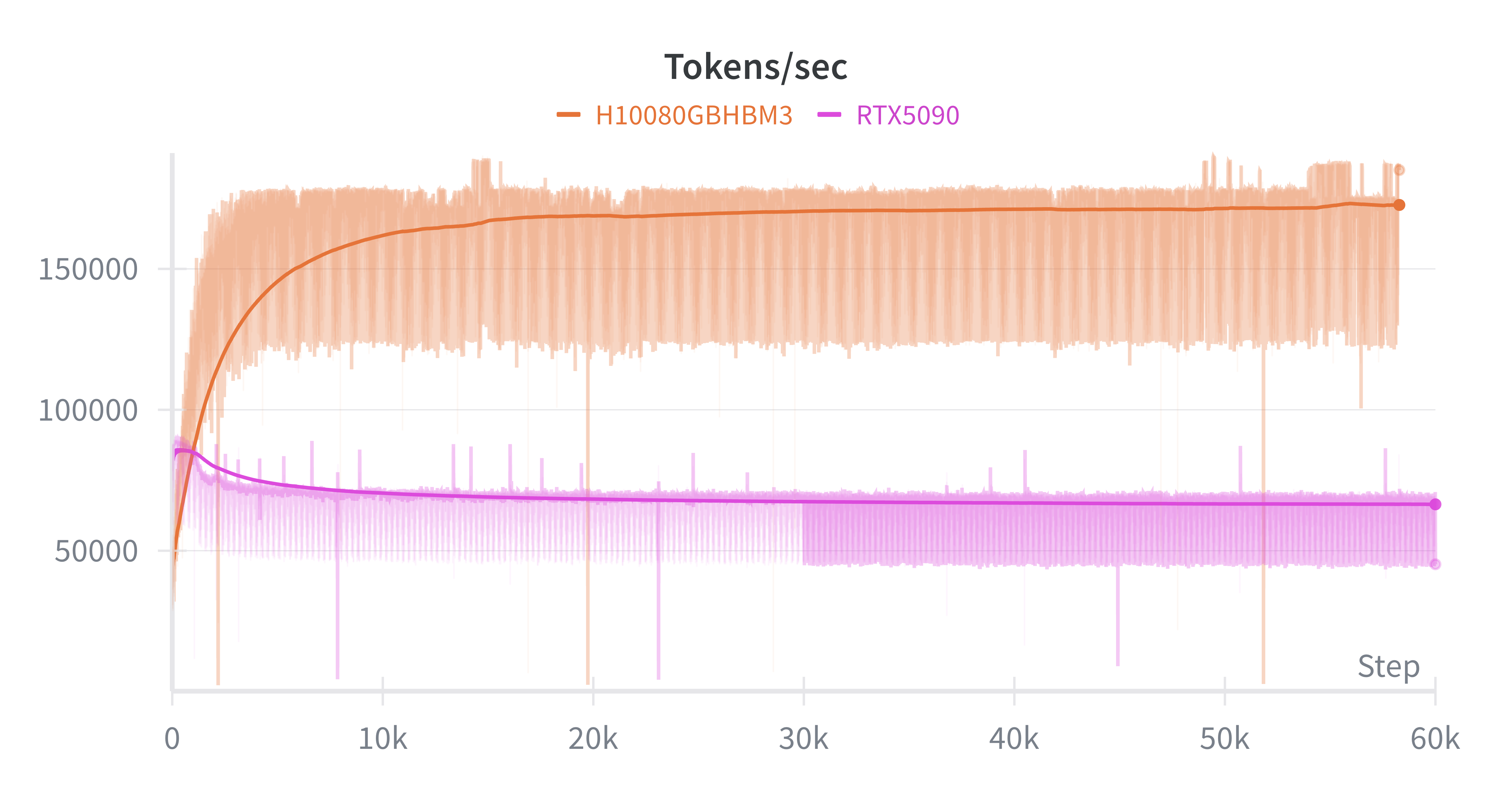
I also compared full precision vs AMP (bfloat16/float16). AMP improved throughput by \(>1.5\times\) with no measurable loss in final performance, though it slightly reduced stability (more frequent gradient spikes without clipping).
Datasets: TinyStories and OpenWebText (CS336 variant).
Model sweep (limited by GPU memory).
- \(d_{\text{model}}\): \(512 \to 1536\)
- \(d_{\text{ff}}: 4\times d_{\text{model}}\) (non-gated) and \(\approx \tfrac{8}{3} d_{\text{model}}\) (gated)
- \(N_{\text{layers}}\): up to \(16\)
- \(N_{\text{heads}}\): \(4, 8, 16\)
- Context length: \(128\to 512\)
Training Loop & Optimizer
I evaluated Adam, AdamW, Adan, Lion, and a Lion-style “trust ratio” hybrid.
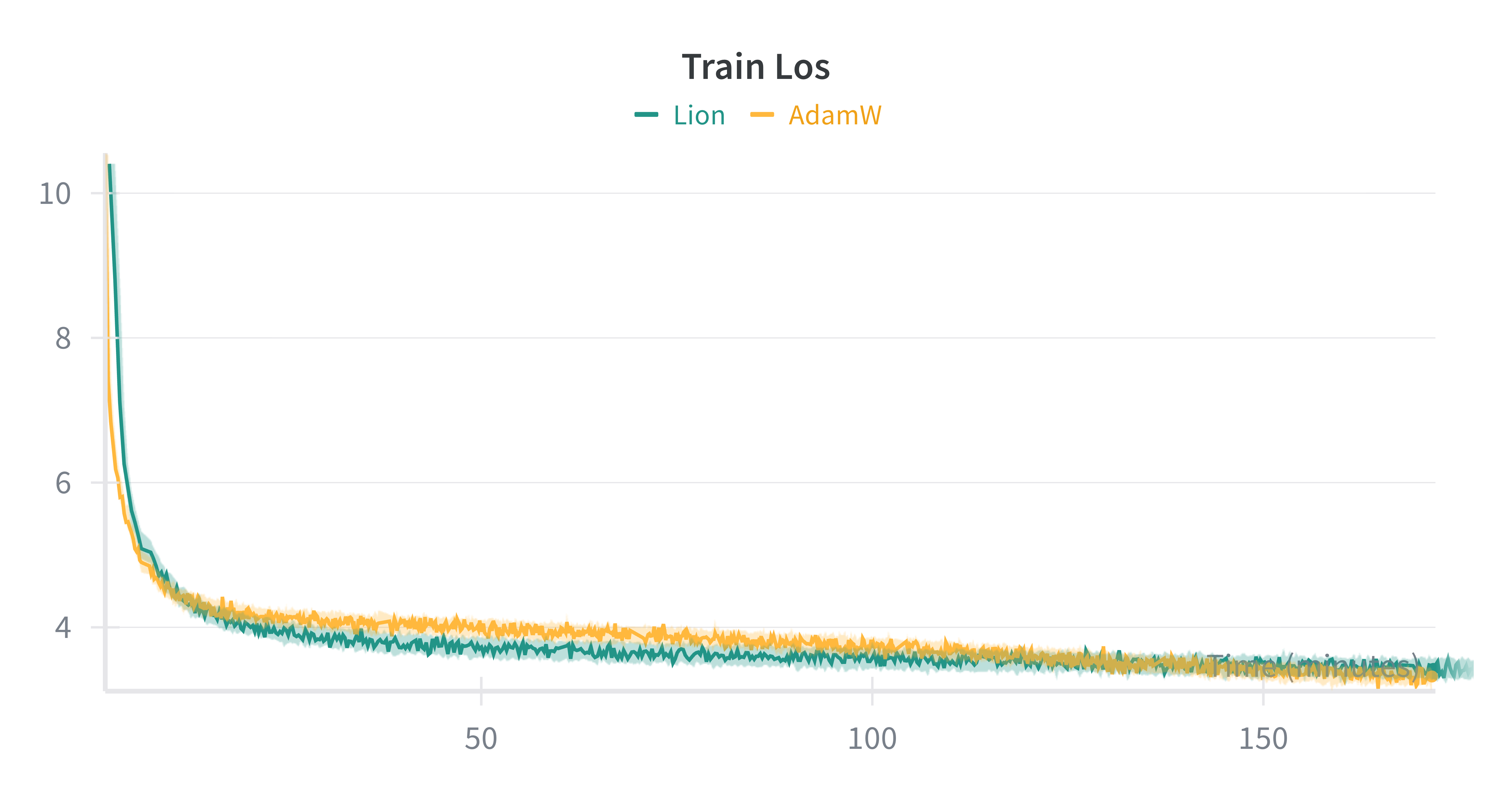
- Lion vs AdamW. Lion consistently reached low loss faster on small models, but often plateaued earlier—likely due to its non-adaptive updates. AdamW remained more consistent late in training. A Lion + trust-ratio variant showed promise but needs deeper study.
- Schedules. Warmup + cosine worked best across the board. I tested several \(\text{lr}{\min}/\text{lr}{\max}\) ratios and settled on \(1/10\) for most of the experiments; this wasn’t especially sensitive.
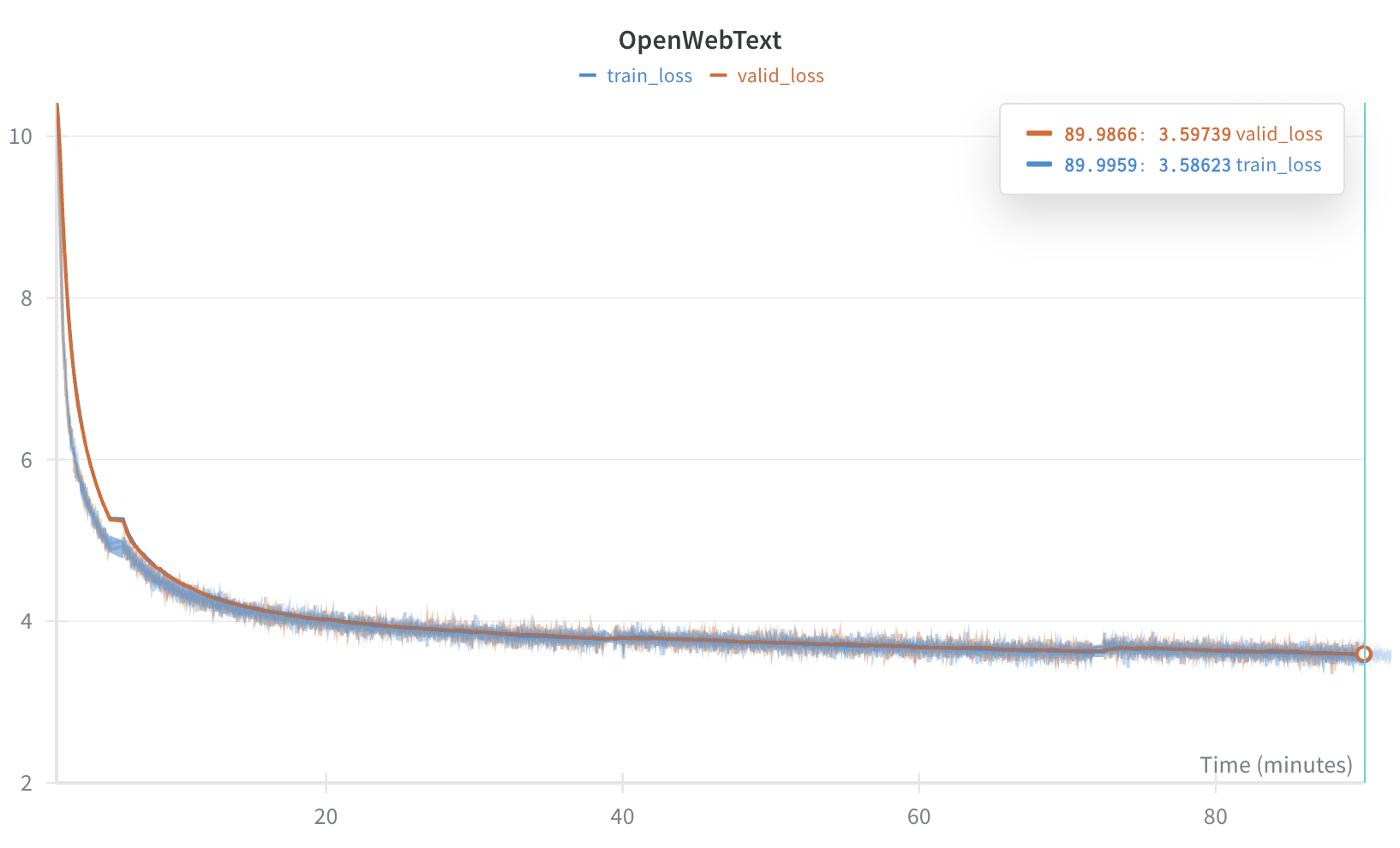
Example Run (OpenWebText, Small Scale)
\(\approx 90\) min. on H100 80 GB HBM3 Config: \(12\) layers, \(16\) heads, \(d_{\text{model}}=1024\), context $256$, batch \(64\), RMSNorm (applied both before and after each block).
Optimizer: Lion (\(\beta_1=\beta_2=0.92\)); cosine schedule with \(\text{lr}{\max}=1\text{e-}4, \text{lr}{\min}=1\text{e-}6\); \(100\) warmup steps; weight decay \(= 0.1\); z-loss = \(1\text{e-}4\). Tokens processed: ~1.6 B.
AdamW vs Lion (same hyperparameters)
Takeaways
What actually moved the needle (small scale):
- Lion accelerated early convergence; AdamW was steadier later.
- AMP provided a clear speed boost with no quality loss (use stability tricks).
- torch.compile nearly doubled training speed - optimization matters (more in following posts).
- Picking the right width (\(d_\text{model}\)) improved GPU utilization and throughput.
- Key stability factors: proper init, gradient clipping, logits scaling/clamp before softmax, Z-loss.
What mattered less (in this regime):
- Exact learning rate (under warmup+cosine and clipping) and optimizer choice (except Lion) had minor impact.
- Weight tying - no performance gain but requires to lower embedding init std (\(1.0 \to 0.02\)) to avoid exploding gradients.
- RMSNorm vs LayerNorm (negligible difference here).
- Activation choice (GELU vs SwiGLU vs SiLu vs squared ReLU) — minimal impact for small models.
Below: convergence comparison with different initialization std values for token embeddings.
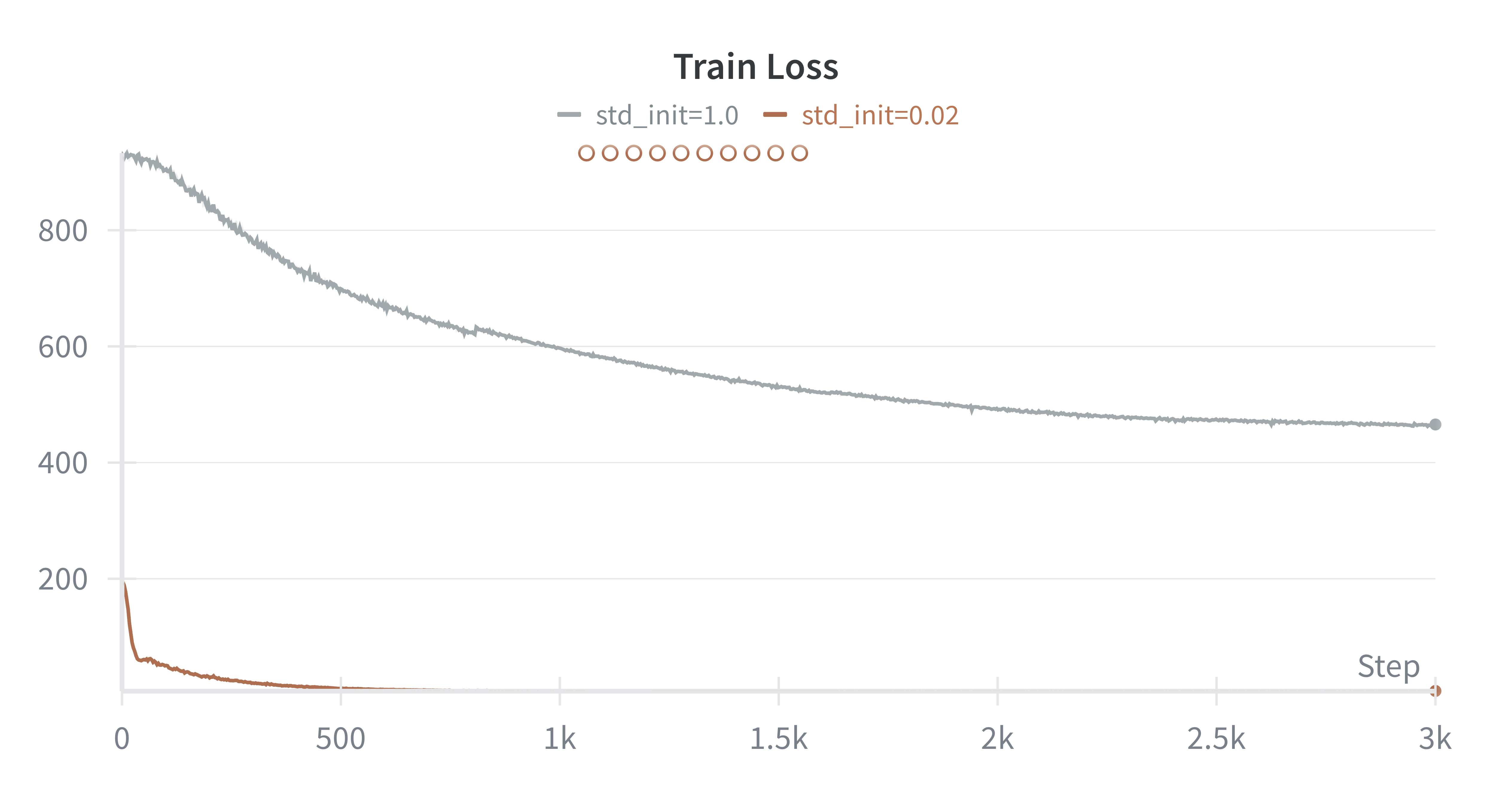
Initialization scale turned out to be one of the most sensitive hyperparameters for stable convergence.
Generation example
Below is an example of text generation from a model trained on the TinyStories dataset:
Prompt:
"Once upon a time"

Generation:
" , there was a little girl named Lucy. She loved to visit her aunt who lived in a small house. One day, Lucy went to visit her aunt and uncle. They had a big, red door that she used to keep her house safe.
When Lucy went inside, she saw her aunt waiting for her. She gave her a big hug and said, 'Thank you, Lucy, for coming to visit me!' Her aunt smiled and said, "You're welcome, Lucy. I hope you enjoy your visit."
From that day on, Lucy visited her aunt every day. They played games, ate yummy food, and had lots of fun together. And they all lived happily ever after."
Model configuration:
- Embedding dimenson: \(d_{\text{model}} = 512\)
- FFN hidden dimension: \(d_{\text{ff}} = 1344\) (or \(\approx \tfrac{8}{3} d_{\text{model}}\))
- Number of layers: \(N_{\text{layers}} = 4\)
- Number of heads: \(N_{\text{heads}} = 16\)
- Context length: \(256\)
- Activation: SwiGLU
- Initialization: Xavier
- Normalization: Post-layer
- Weight tying: Disabled
Conclusion & Next Steps
In this post, I described how I implemented a mini LLM from scratch and trained it on TinyStories and OpenWebText. I walked through core design patterns and a few newer twists. I was able to reproduce key behaviors observed in large models — most notably the importance of proper initialization, the stabilizing role of Z-loss, and how Lion accelerates early convergence while adaptive optimizers remain stronger at scale.
Next, I plan to explore optimization techniques that matter in practice:
- Memory-efficient inference: KV-cache compression and attention variants (MQA, GQA, MLA).
- Distributed training approaches: DDP, FSDP, ZeRO, and their trade-offs.
- FlashAttention-2 in Triton: from intuition to implementation.
- Mixture-of-Experts (MoE): gating, routing, load-balancing, and stability.
Enjoy Reading This Article?
Here are some more articles you might like to read next: