Attention at Inference: Arithmetic Intensity & KV Cache
In this post I cover the arithmetic intensity of Multi-Head Attention (MHA) during training and inference, and how modern variants raise intensity and reduce memory movements.
I’ll discuss:
- KV Cache
- Multi-Query Attention (MQA)
- Grouped Query Attention (GQA)
- Multi-Head Latent Attention (MLA)
Introduction
I’ll use standard Transformer notation. Let batch \(b\), query sequence length \(n_q\), key/value sequence length \(n_{kv}\), model dim \(d\), number of heads \(h\), head dim \(d_h=d/h\).
Let \(d_q, d_k, d_v\) be projections dimensions of queries (\(\mathbf{Q}\)), keys (\(\mathbf{K}\)), and values (\(\mathbf{V}\)) respectively.
For simplicity, I assume \(d_q=d_k=d_v=d\).
Inputs:
- Sequences: \(X \in \mathbb{R}^{b\times n_q \times d}, Z \in \mathbb{R}^{b \times n_{kv} \times d}\)
- Projections: \(W_Q \in \mathbb{R}^{d\times d_q}, W_K \in \mathbb{R}^{d\times d_k}, W_V \in \mathbb{R}^{d\times d_v}, W_O \in \mathbb{R}^{d_v\times d}\)
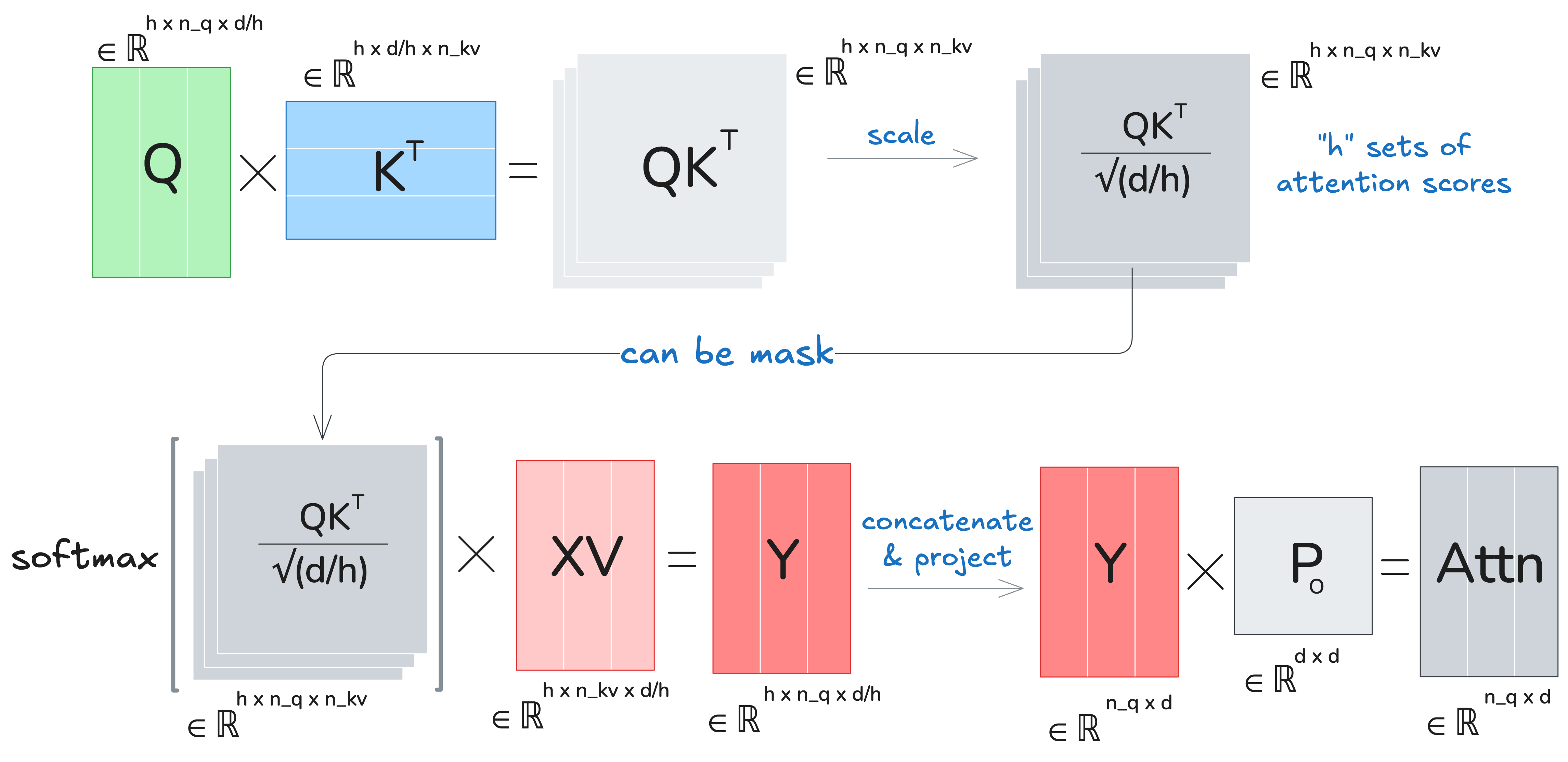
Scaled attention (per layer):
- Project: \(Q = X W_Q,\quad K = Z W_K,\quad V = Z W_V\)
- Scores and Weights \(S= \frac{QK^\top}{\sqrt{d_h}},\quad Y = \operatorname{softmax}(S)\)
- Attention: \(O = \operatorname{Concat}_H(Y)\, W_O\).
Schema:
I’ll use arithmetic intensity (\(\mathbb{AI}\)) as \(\frac{\mathbb{FLOPs}}{\mathbb{total\ memory\ accessed}}\). Higher \(\mathbb{AI} ⇒\) less memory-bound.
Scope:
- Training: full sequence, parallel dense matrix multiplications; $n_q = n_{kv} = n$.
- Inference: single-token step t with a KV cache; \(n_q = 1, n_{kv} = n\).
Assumption:
Model dim \(d\) often scales with context \(n\); I’ll assume \(d=\Theta(n)\).
Shazeer (2019) assumed \(n\ll d\) in MQA, but today’s long contexts make \(n\) comparable to \(d\).
MHA Arithmetic Intensity during Training
The FLOPs in Multi-Head Attention (MHA) are dominated by matrix multiplications:
- Projections \(\mathbf{Q, K, V}\): \(3 \times 2\times b\times n\times d^2=6bnd^2\)
- Scores computation \(\mathbf{S}\): \(2 \times b\times h\times n\times (d/h)\times n=2bn^2d\)
- Attention output \(\mathbf{Y}\): \(2 \times b\times h\times n^2\times (d/h)\)
- Final projection \(\mathbf{O}\): \(2bnd^2\)
Total \(\mathbb{FLOPs} = O(bn^2d+bnd^2) \approx O(bn^2d)\) if \(d = \Theta(n)\).
Memory accesses include all tensor reads/writes in High Bandwidth Memory (HBM), and equal the size of all tensors involved:
- \(\mathbf{X, Z, Q, K, V, O, Y}\): \(O(bnd)\)
- Scores and attention weights (if materialized in HBM) \(\mathbf{S}\): \(O(bhn^2)\)
- Projection matrices \(\mathbf{P_Q, P_K, P_V, P_O}\): \(O(d^2)\)
Total \(\mathbb{total\ memory\ accessed} = O(bnd + bhn^2 +d^2)\).
Arithmetic Intensity:
Dividing FLOPs by memory accesses gives:
\(\mathbb{AI} = O(\frac{bn^2d}{bnd+bhn^2+d^2}) = O((\frac{1}{n}+\frac{h}{d}+\frac{d}{bn^2})^{-1})=O((\frac{1}{n}+\frac{1}{d_h}+\frac{d}{bn^2})^{-1})\), where \(d_h = d/h\) is the dimension per head.
Assuming \(d = \Theta(n)\), this simplifies to \(O\!\big((\tfrac{1}{d_h} + (1+\tfrac{1}{b})\tfrac{1}{n})^{-1}\big)\).
Takeaway:
In practice the \(1/d_h\) term usually dominates (especially for a long sequences). Since, $1/d_h$ is quite small, the arithmetic intensity remains high.
During training, MHA has high arithmetic intensity, meaning it is FLOPs-bound rather than memory-bound - which is good for modern GPUs.
KV Cache
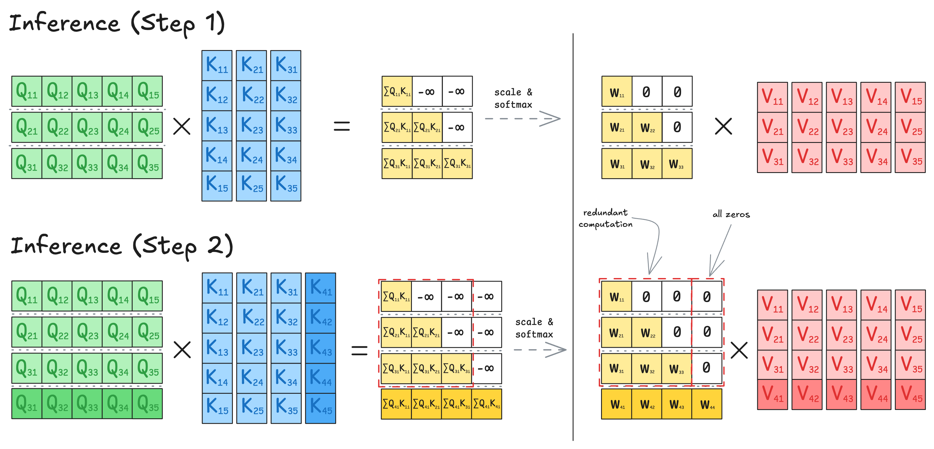
Inference is incremental - at step \(t\), the model attends to tokens \(1{:}t\). Naively, we would require recomputing all previous \(\mathbf{K}_{1:t}, \mathbf{V}_{1:t}\) at every step.
Instead, we can cache the key and value projections from earlier steps and append only the latest \(\mathbf{K}_t, \mathbf{V}_t\). This avoids redundant computation and allows us to reuse past results.
This technique is called the KV cache — and it’s essential for fast, efficient inference in LLMs.
Compute impact:
I’ll analyze the per-layer compute (\(\mathbb{FLOPs}\)) cost (in big-O) over the full decode of a sequence of length \(n\).
Without KV cache: At every step \(t\), we:
- Recompute all \(\mathbf{K}_{1:t}, \mathbf{V}_{1:t}\) (projections)
- Compute full attention scores \(Q_t K_{1{:}t}^\top\) and softmax weights
With KV cache:
- Each \(\mathbf{K}_t, \mathbf{V}_t\) is computed once and stored
- At each step, we compute only the last row of \(QK^\top\) and apply softmax over it.
So we reduce decode-time compute by an order of magnitude in \(n\).
However, the cost now shifts to memory bandwidth. At each step \(t\), we must read all cached \(\mathbf{K}, \mathbf{V}\) of width \(d_h\) per head, which stresses HBM throughput - especially at large context lengths.
Minimal implementation:
# In __init__
if kv_cache:
    # Works for batch_size == 1. Consider register_buffer for persistence.
    self.register_buffer(
        "cache_k",
        torch.empty((1, self.num_heads_kv, self.cntx, self.d_qk), device = device, dtype = dtype),
        persistent = False
    )
    self.register_buffer(
        "cache_v",
        torch.empty((1, self.num_heads_kv, self.cntx, self.d_v), device = device, dtype = dtype),
        persistent = False
    )
    self.start, self.kv_cache_len = 0, 0

# Inside 'get_proj_kv'
if hasattr(self, "kv_cache_len"):
    assert batch_size == 1, f"Currently support batch_size = 1, but provided {batch_size}"

    # populate KV Cache (NOTE: for now it works only for batch_size = 1)
    if self.kv_cache_len == 0:
        k = self.P_K(x)  # batch_size x seq_len x (h d_qk)
        k = rearrange(k, "... seq_len (h d_qk) -> ... h seq_len d_qk", h = self.num_heads_kv)
        self.cache_k[:, :, :seq_len,:] = k
        if with_rope and self.rope is not None:
            k = self.rope(k, token_positions = token_positions)

        v = self.P_V(x)  # batch_size x seq_len x (h d_v)
        v = rearrange(v, "... seq_len (h d_v) -> ... h seq_len d_v", h = self.num_heads_kv)
        self.cache_v[:, :, :seq_len,:] = v
        self.kv_cache_len = seq_len
    else:
        assert seq_len == 1, "You don't need to provide the whole input after prefill"

        # 1) choose write position + update ring pointers
        if self.kv_cache_len < self.cntx:
            pos = self.kv_cache_len              # append at end
            self.kv_cache_len += 1
        else:
            pos = self.start               # overwrite oldest
            self.start = (self.start + 1) % self.cntx

        # 2) write new K/V
        k_new = self.P_K(x)
        k_new = rearrange(k_new, "... seq_len (h d_qk) -> ... h seq_len d_qk", h=self.num_heads_kv)
        self.cache_k[:, :, pos:pos+1, :] = k_new

        v_new = self.P_V(x)
        v_new = rearrange(v_new, "... seq_len (h d_v) -> ... h seq_len d_v", h=self.num_heads_kv)
        self.cache_v[:, :, pos:pos+1, :] = v_new

        # 3) read logical window (oldest -> newest)
        idx = (self.start + torch.arange(self.kv_cache_len, device=x.device)) % self.cntx
        k = self.cache_k[:, :, idx, :]
        v = self.cache_v[:, :, idx, :]

        # 4) apply RoPE to the logical window
        if with_rope and self.rope is not None:
            k = self.rope(k, token_positions=token_positions)
With KV cache implemented, inference on my TinyStory model became 4× faster - reducing average per-token latency from \(16.91\) ms to \(4.21\) ms, measured on an Apple M2 over 150 generation steps. Prefill step is not included in calculation.
The bottleneck has shifted: as sequence length grows, KV cache memory usage and HBM bandwidth are the main constraints.
MHA Arithmetic Intensity during Inference
Once we adopt a KV cache, the total FLOPs across an entire inference pass of length \(n\) match the forward pass during training: \(\mathbb{FLOPs} = \Theta(bn^2d+bnd^2) \approx \Theta (bn^2d)\) if \(d = \Theta(n)\).
However, memory accesses per step change significantly:
- New token embeddings / outputs (\(\mathbf{X, Q, O, Y}\)): \(\Theta(bd)\)
- KV reads (\(\mathbf{K, V}\)): \(\Theta(btd_\text{kv})\) (for MHA, \(d_\text{kv}=d\))
- Attention scores / weights (if materialized in HBM) (\(\mathbf{S}\)): \(\Theta(bht)\)
- Projection weights (\(\mathbf{P_Q, P_K, P_V, P_O}\)): \(\Theta(d^2)\)
Summing over all steps \(t = 1 \dots n\) gives:
\(\Theta\!\Big(\sum_{t=1}^n (b d + b t d_{\text{kv}} + b h t + d^2)\Big) = \Theta(b n^2 d_{\text{kv}} + b n^2 h + n d^2) \overset{\text{MHA}}{=} \Theta(b n^2 d + n d^2)\) (typically $d \gg h$).
Arithmetic intensity:
\(\mathbb{AI} = \Theta(\frac{bn^2d + bnd^2}{bn^2d+nd^2}) = \Theta(\frac{bn+bd}{bn+d})\).
If we assume \(d=\Theta(n)\) (e.g. \(n=c \cdot d\)), this simplifies to: \(\mathbb{AI}\;=\;\Theta\!\left(\frac{b(c+1)}{\,bc+1\,}\right)\;=\;\Theta(1)\).
Implication:
When batch size \(b \approx 1\) (typical for autoregressive decoding), arithmetic intensity approaches \(\mathbb{AI} \approx 1\). This makes inference memory-bound, with HBM bandwidth becoming the dominant bottleneck - especially at large context lengths.
MQA and GQA
To improve arithmetic intensity and reduce KV cache memory,
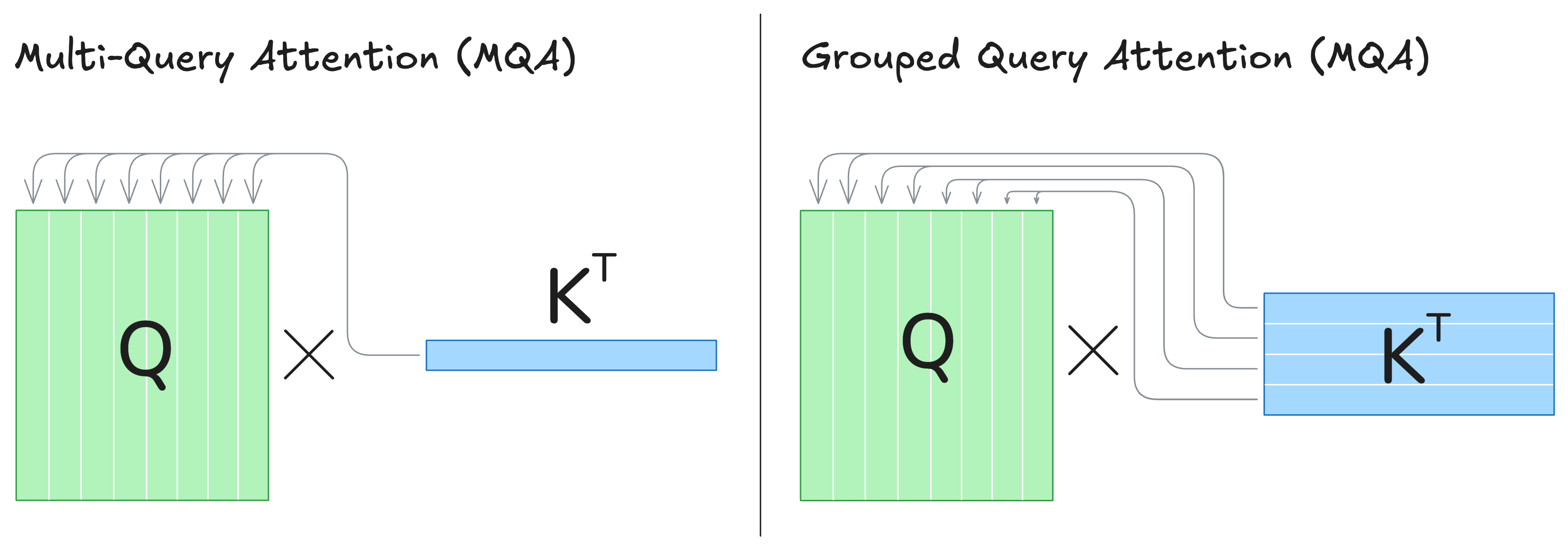
- MQA (Shazeer, 2019) shares K, V across all query heads - using just one KV head, broadcast to all Q-heads.
- GQA (Ainslie et al., 2023) is the middle ground: share K,V across groups of query heads (e.g., 2, 4, 8 Q-heads per KV).
Schema.
Below is a visual for how Query–Key interaction changes under MQA and GQA (V is analogous)
FLOPs:
The total FLOPs asymptotics across inference remain unchanged:
\(\mathbb{FLOPs} = \Theta(bn^2d+bnd^2) \approx \Theta (bn^2d)\) if \(d = \Theta(n)\).
Set the key-value head dimension:
\(d_{\text{kv}}=\begin{cases} d/h & \text{MQA}\\ d/G & \text{GQA} \end{cases}\)
Memory accesses (after \(n\) steps):
\(\Theta\!\Big(\sum_{t=1}^n (b d + b t d_{\text{kv}} + b h t + d^2)\Big) = \Theta(bnd + b n^2 d_{\text{kv}} + b n^2 h + n d^2)\)
In practice, \(bd\) and \(bn^2 h\) are less critical - e.g., fused attention kernels often hide the \(bn^2 h\) term.
So we focus on: \(\begin{cases} \Theta\!\left(bn^2d/h + nd^2\right) & \text{MQA}\\[6pt] \Theta\!\left(bn^2d/G + nd^2\right) & \text{GQA} \end{cases}\)
Arithmetic intensity:
We define:
\(\mathbb{AI} = \Theta\!\left(\frac{b n^2 d + b n d^2}{\,b n^2 d_{\text{kv}} + n d^2\,}\right)\)
which simplifies to
\(\begin{cases} \Theta\!\left(\dfrac{b(n+d)}{b n / h + d}\right)=\Theta\!\left(h \cdot \dfrac{bn+bd}{bn+hd}\right) & \text{(MQA)}\\[6pt] \Theta\!\left(\dfrac{b(n+d)}{b n / G + d}\right)=\Theta\!\left(G \cdot \dfrac{bn+bd}{bn+Gd}\right) & \text{(GQA)} \end{cases}\)
If batch size is large enough (\(b \gg h\) or \(G\)) and \(n \gg d\), this becomes:
\(\mathbb{AI}= \begin{cases} \Theta\!\left(h\right) & \text{(MQA)}\\[6pt] \Theta\!\left(G\right) & \text{(GQA)} \end{cases}\)
Key insight:
Even without these assumptions, reducing \(d_{\text{kv}}\) shrinks KV cache memory and bandwidth by:
- \(\times h\) (MQA)
- \(\times G\) (GQA)
This is why MQA and GQA dramatically reduce inference latency and memory load.
Empirical Results:
- MQA provides the biggest gains in speed and memory.
- GQA trades off a bit of performance to recover model quality, and often strikes a good balance - with latency close to MQA and quality close to MHA.
To implement GQA, we need two small adjustments in scaled dot product attention; MQA broadcasts on the fly.
def scaled_dot_product_attention(Q: torch.Tensor, K: torch.Tensor, V: torch.Tensor, mask: torch.Tensor | None):
    """
    Q:  (batch_size, ..., seq_len_q, d_qk) # seq_len_q = 1 for KV Cache
    K:  (batch_size, ..., seq_len_kv, d_qk)
    V:  (batch_size, ..., seq_len_kv, d_v)
    """
    d_qk = K.shape[-1]
    H_q, H_kv = Q.shape[1], K.shape[1]

    # Grouped-Query Attention reshape
    if H_q > H_kv and H_kv > 1: # GQA
        Q = rearrange(Q, "... (h_kv r) seq_len_q d_qk -> ... h_kv r seq_len_q d_qk", h_kv = H_kv)
        K = rearrange(K, "... h_kv seq_len_kv d_qk -> ... h_kv 1 seq_len_kv d_qk")
        V = rearrange(V, "... h_kv seq_len_kv d_v -> ... h_kv 1 seq_len_kv d_v")

    # Compute scores
    scores = einsum(Q, K, "... seq_len_q d_qk, ... seq_len_kv d_qk -> ... seq_len_q seq_len_kv")
    scores = scores.clamp(min = -80, max=80.0) # NOTE: might be better after rescaling

    # Compute masking
    if mask is not None:
        scores = scores.masked_fill(~mask, float('-inf'))

    # Compute weights
    weights = softmax(scores / (d_qk ** 0.5), dim = -1)

    # Compute attention
    attn = einsum(weights, V, "... seq_len_q seq_len_kv, ... seq_len_kv d_v -> ... seq_len_q d_v")
    # Rearrange GQA to (B, H, S, d_h)
    if H_q > H_kv and H_kv > 1: # GQA
        attn = rearrange(attn, "... h_kv r seq_len_q d_h -> ... (h_kv r) seq_len_q d_h")
    return attn
MLA
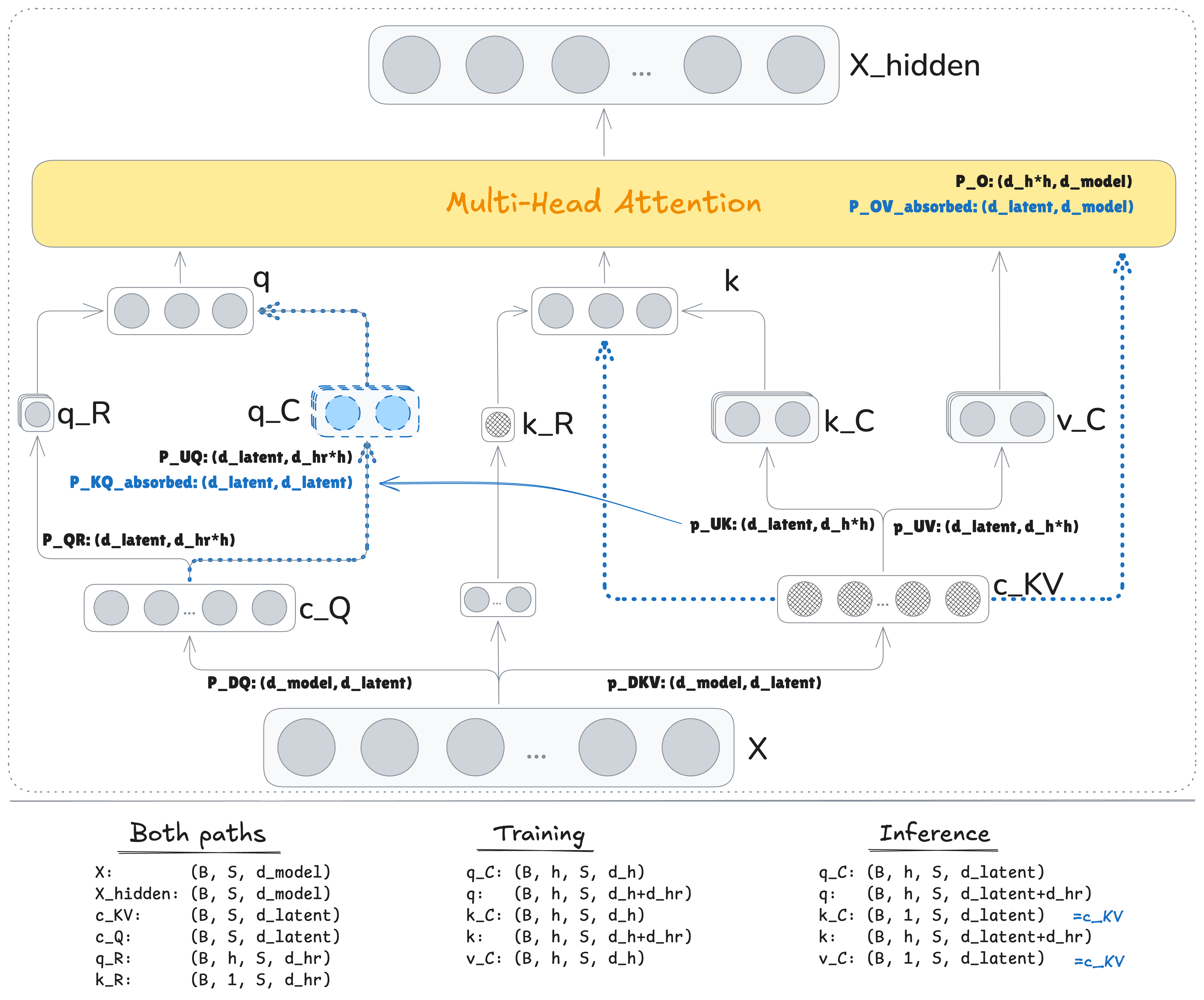
DeepSeek V2(DeepSeek AI, 2024) tackles the large KV cache problem from a different angle: keep all heads, but shrink the per-token cache using a low-rank latent representation. The idea is LoRA-style:
- Down-project the token hidden state \(h_t\in\mathbb{R}^d\) to a small latent vector \(c_t^{\mathrm{KV}} \in \mathbb{R}^{d_c}\): \(c_t^{\mathrm{KV}} = W_{\mathrm{DKV}}h_t, \quad W_{\mathrm{DKV}} \in \mathbb{R}^{d_c \times d}, \quad d_c \ll d.\)
- Up-project this latent to get keys and values:
\(K_t = W_{\mathrm{UK}}\,c_t^{\mathrm{KV}},\quad V_t = W_{\mathrm{UV}}\,c_t^{\mathrm{KV}},\qquad W_{\mathrm{UK}},W_{\mathrm{UV}}\in\mathbb{R}^{(d_h n_h)\times d_c}\),
where \(d_h\) is the per-head dimension and \(n_h\) is the number of heads. - Cache only the small latent \(c_t^\mathrm{KV}\) (width \(d_c\)) per token. During inference, pre-fold:
\(\hat W_\mathrm{Q} = W_\text{UK}^\top W_\mathrm{Q} ,\ \hat W^\mathrm{O} = W_\text{UV} W_\mathrm{O}\),
so attention can run in latent space and decode once at the end.
This dramatically reduces KV cache - from \(2d_h n_h\) down to just \(d_c\) elements per token per layer.
RoPE Incompatibility
There’s one problem: RoPE. Normally, RoPE is applied a position-dependent rotation after projection: \(\tilde Q_t=R(t)\,(W_Q h_t),\ \tilde K_j=R(j)\,(W_K h_j)\).
But with MLA, that rotation sits between \(W_\mathrm{Q}\) and \(W_\mathrm{UK}^\top\). Since matmul isn’t commutative (\(W_\mathrm{Q}^\top\,R(t)\,W_\mathrm{UK} \;\neq\; (W_\mathrm{Q}^\top W_\mathrm{UK})\,R(t)\)) - we can’t absorb \(W_\mathrm{UK}\) into \(W_\mathrm{Q}\) once and reuse it. That’s the core incompatibility flagged in the DeepSeek V2 paper.
The Fix: Decouple RoPE
Keep content in the latent and carry position via a tiny side stream:
DeepSeek proposes a neat workaround:
- Compute a side positional embedding \(k^\mathrm{R}_t\) (e.g., using RoPE on one small head).
- Concatenate it with the latent: \([c_t^{\mathrm{KV}} \,\|\, k^\mathrm{R}_t]\).
- Use a projection \(W_{\mathrm{UK}}\) to get a position-aware key.
During inference, only the new tuple \((c_t^{\mathrm{KV}}, k_t^R)\) is appended. Previous latents remain untouched.
Details match the schema (adapted from DeepSeek):
My MLA implementation is available in the repo — see the class MultiHeadLatentAttention.
The table below summarizes KV cache per token and relative performance of attention variants (adapted from DeepSeek V2):
| Attention Mechanism | KV Cache per Token | Capability |
|---|---|---|
| Multi-Head Attention (MHA) | $2n_h d_h l$ | Strong |
| Grouped-Query Attention (GQA) | $2n_g d_h l$ | Moderate |
| Multi-Query Attention (MQA) | $2 d_h l$ | Weak |
| Multi-Head Latent Attention (MLA) | $(d_c+d_h^R) l \approx \frac{9}{2} d_h l$ | Weak |
Inference Benchmarks
I benchmarked inference performance for MHA, GQA, MQA, and MLA — both with and without KV-Cache - on three devices: Apple M2, AMD Ryzen Threadripper 7960X (24 cores), and NVIDIA RTX 5090.
The model was trained on the TinyStories dataset with the following architecture:
- \(d_{\text{model}} = 512\).
- \(d_{\text{ff}} = 1344 (\approx \tfrac{8}{3})\) (FFN with SwiGLU)
- \(N_{\text{layers}}=4\).
- \(N_{\text{heads}}=16\) (KV heads depend on the type of attention)
- Context length: \(256\).
I tested inference at maximum context lengths of 64 and 256, initial prompt was always “Once upon a time”. The shorter sequence length yielded 5–10% lower latency, but all reported results below use 256 for consistency.
Apple M2
Inference latency (in ms) for each attention mechanism, with and without KV cache.
| Attention Mechanism | Prefill (no KV), ms | Avg. Gen (no KV), ms | Prefill (KV), ms | Avg. Gen (KV), ms |
|---|---|---|---|---|
| MHA | 28.84 | 16.76 | 25.03 | 4.36 |
| GQA, $$G=4$$ | 29.09 | 15.39 | 24.39 | 3.92 |
| MQA | 26.9 | 14.45 | 20.05 | 3.99 |
| MLA, $d_\text{latent} = 64$ | 25.14 | 15.93 | 29.46 | 4.55 |
| MLA, $d_\text{latent} = 128$ | 28.23 | 15.55 | 32.06 | 4.40 |
AMD Ryzen Threadripper 7960X
Inference latency (in ms) for each attention mechanism, with and without KV cache.
| Attention Mechanism | Prefill (no KV), ms | Avg. Gen (no KV), ms | Prefill (KV), ms | Avg. Gen (KV), ms |
|---|---|---|---|---|
| MHA | 8.35 | 13.42 | 8.38 | 8.11 |
| GQA, $$G=4$$ | 8.87 | 13.00 | 24.39 | 3.92 |
| MQA | 7.6 | 12.71 | 7.75 | 7.61 |
| MLA, $d_\text{latent} = 64$ | 8.27 | 13.36 | 9.29 | 7.30 |
| MLA, $d_\text{latent} = 128$ | 9.91 | 13.07 | 10.27 | 7.99 |
RTX5090
Inference latency (in ms) for each attention mechanism, with and without KV cache.
| Attention Mechanism | Prefill (no KV), ms | Avg. Gen (no KV), ms | Prefill (KV), ms | Avg. Gen (KV), ms |
|---|---|---|---|---|
| MHA | 196.92 | 4.09 | 196.29 | 4.03 |
| GQA, $$G=4$$ | 194.49 | 4.16 | 198.87 | 4.36 |
| MQA | 206.58 | 3.93 | 203.8 | 4.19 |
| MLA, $d_\text{latent} = 64$ | 195.6 | 4.72 | 211.9 | 4.49 |
| MLA, $d_\text{latent} = 128$ | 197.58 | 4.78 | 211.68 | 4.51 |
Below are plots comparing per-step generation latency over time for MHA - with and without KV Cache — after the prefill phase. Measurements were taken on Apple M2.
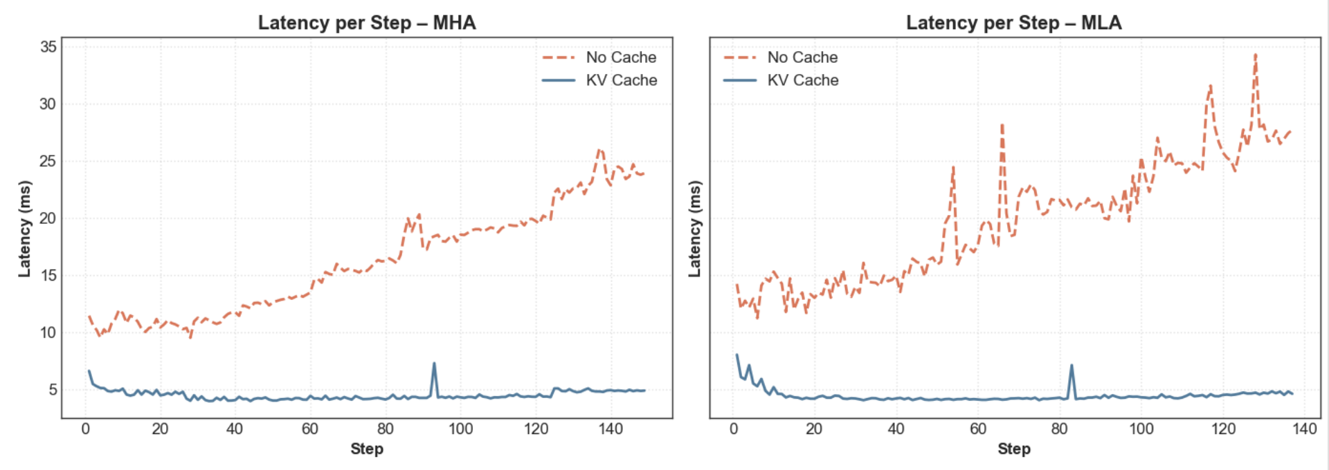
Without KV cache, latency grows steadily with sequence length, since at every generation step the model must recompute attention over all previously generated tokens.
Bonus: Determinism and Floating-Point Weirdness
When benchmarking my implementations of MHA, GQA, MQA, and MLA, I wanted to ensure that runs with and without KV cache produced identical output. Since LLM inference typically includes sampling, I set \(\text{top-k} = 1\) to make the generation deterministic.
I was able to get exactly the same outputs for MHA, MQA, and GQA. However, for MLA, the outputs between KV-cache and non-KV-cache runs started diverging - but not immediately. The first 31 tokens matched, and differences only began from token 32 onward:
Without Cache:

With KV Cache:

Before diving deeper, I want to highlight a fantastic post by Horace He and Thinking Machines: “Defeating Non-Determinism in LLM Inference”. It offers a detailed exploration of determinism issues — including atomic operations, and kernel-level quirks.
But the most important takeaway for my issue comes right at the start: “The original sin: floating-point non-associativity”.
Which means \(a \times (b \times c) \ne (a \times b) \times c\) when using floating points (most of the time).
I believe that is why my MLA outputs diverged between KV and non-KV runs. In MLA during inference, we pre-fold two matrices:
- \(\hat W_\mathrm{Q} = W_\text{UK}^\top W_\mathrm{Q}\).
- \(\hat W^\mathrm{O} = W_\text{UV} W_\mathrm{O}\).
This changes the order of floating-point operations, which is enough to cause minor numerical drift. Over multiple decoding steps, even small differences can amplify - eventually shifting top-1 choices.
In other words: both versions are “correct” — just a subtle reminder that numerical reproducibility in deep learning is fragile, especially with architectural changes that affect operation order.
…
Conclusion
In this blog, I walked through the concept of KV Cache and explored techniques to reduce its memory overhead. Specifically, I explained and implemented MQA, GQA, and MLA - alternative attention mechanisms designed for more efficient inference. I also benchmarked their performance across different hardware setups
The experiments confirm that KV Cache brings substantial performance improvements:
- On Apple M2 and Ryzen CPU, enabling KV Cache reduced average generation latency by 2–4×, making it a crucial optimization for low-power or general-purpose environments.
- On RTX 5090, the prefill phase is extremely long - likely due to data movement overheads or kernel warm-up costs.
- KV Cache showed little or no gain on GPU for short sequences (\(\geq 150\) tokens) This suggests the GPU is underutilized at this scale, and inference becomes memory-bound bound rather than compute-bound.
Enjoy Reading This Article?
Here are some more articles you might like to read next: