Gradient-Based Optimization: Theory, Practice, and Evolution
In this post, I’ll break down the core ideas behind popular optimizers used in Deep Learning. Starting with Vanilla Gradient descent, I’ll explore how momentum, adaptive learning rates, and their combinations (like Adam) help models converge faster and more reliably — and the intuition behind each step. Finally, I’ll mention briefly latest developments.
Vanilla Gradient Descent
Core Idea: Move weights in the direction of the negative gradient to minimize the loss.
In Deep Learning, the typical goal is to minimize a loss function - we may also call it cost function - over a training dataset.
Gradient Descent is the foundation of most Deep Learning optimizers. In practice, we compute the gradient of loss \(f(W)\) with respect to the model’s weights \(W\) and update iteratively the weights accordingly. On each step, we subtract the gradient of the loss with respect to the weights, scaled by a learning rate:
In Python code, this looks like:
while cond:
    weights_grad = evaluate_gradient(loss_func, data, weights)
    weights -= learning_rate * weights_grad
Each iteration updates weights in the direction that locally reduces the loss. The stopping condition may be a fixed number of steps or a threshold on loss improvement. For instance, in LLMs it is generally iteration over one epoch - over all data one time.
Let’s walk through a concrete example. Suppose: \(W = \begin{bmatrix} w_1\\ w_2 \end{bmatrix}\) is a \(\text{2D}\) vector, and \(f(W) = w_1^2 + bw_2^2 = W^T \begin{bmatrix} 1 & 0\\ 0 & b \end{bmatrix} W\).
Then:
- Minimum: \(\min f(W) = 0\) at \(W = \begin{bmatrix} 0\\ 0 \end{bmatrix}\) (\(\text{argmin}\)).
- Gradient: \(\nabla_W f(W) = \begin{bmatrix} 2w_1\\ 2bw_2 \end{bmatrix}\).
- Update rule: \(W_{k+1} =W_k - \text{lr} * \nabla f(W_k) = \begin{bmatrix} w_1\\ w_2 \end{bmatrix} - \text{lr} \begin{bmatrix} 2w_1\\ 2bw_2 \end{bmatrix} = \begin{bmatrix} (1-2*\text{lr})w_1\\ (1-2*b*\text{lr})w_2 \end{bmatrix}\).
I simulate gradient descent from initial point \(W^0 = \begin{bmatrix} 0.5 \\ 0.5\end{bmatrix}\) with learning rate \(\text{lr} = 0.3\) in two cases (different values of \(b\)):
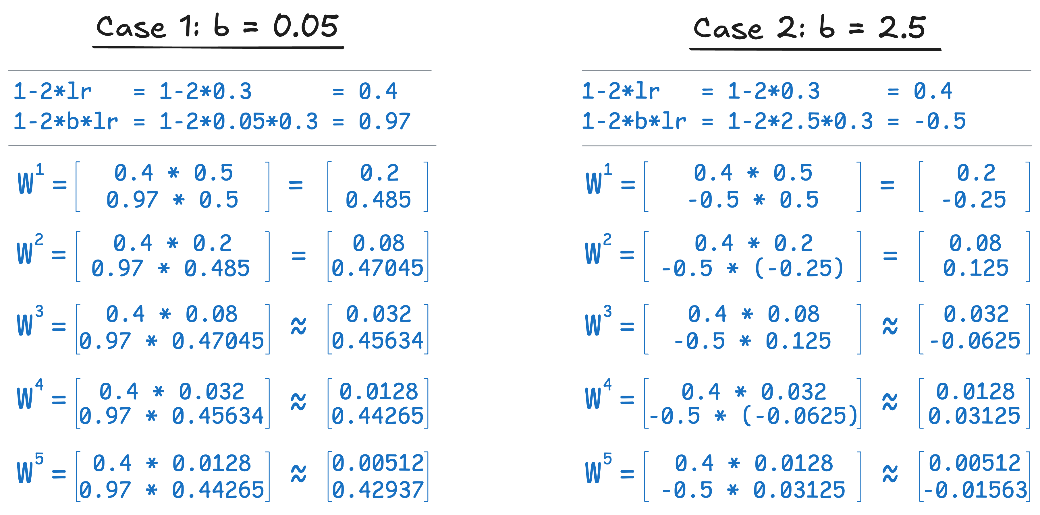
Observation:
- Progress along different dimension can vary dramatically if conditioning is poor.
- The path may “zig-zag” - commonly when the loss landscape is elongated.
Stochastic Gradient Descent
Vanilla Gradient Descent assumes we can compute gradients over the entire dataset at every step. For large datasets, this becomes computationally infeasible.
A more practical alternative is Stochastic Gradient Descent (SGD): Instead of using all data, SGD approximates the gradient using a random mini-batch at each step. This introduces some noise but dramatically improves efficiency and scalability.
while cond:
    batch = sample_batch(data)
    weights_grad = evaluate_gradient(loss_func, batch, weights)
    weights -= learning_rate * weights_grad
Today, almost every optimizer - from SGD+Momentum to Adam, and beyond - is built on this stochastic mini-batch principle.
Challenges with SGD:
-
Noisy behaviour
Gradients computed on a mini-batch fluctuate due to sample variance. It is not always bad in fact — for example, it can be helpful in avoiding sharp local minima. -
Poor conditioning
Loss surface has directions with very different curvature — some steep, others flat. Formally, it means a large ratio between the largest and smallest eigenvalues of the Hessian. As a result, we observe “zig-zag” behaviour and slow convergence in flatter directions.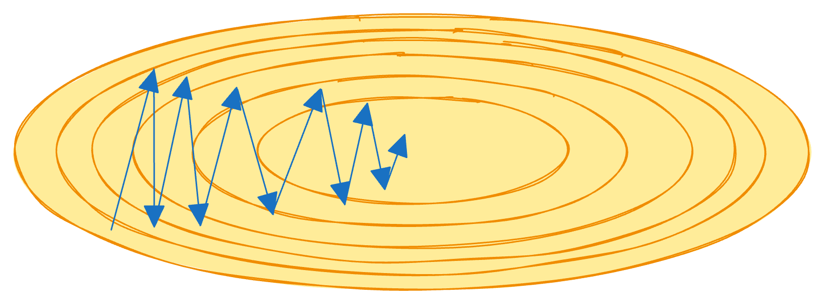
-
Local minima and saddle points
If the gradient vanishes, SGD may stall — even if it’s not a true minimum.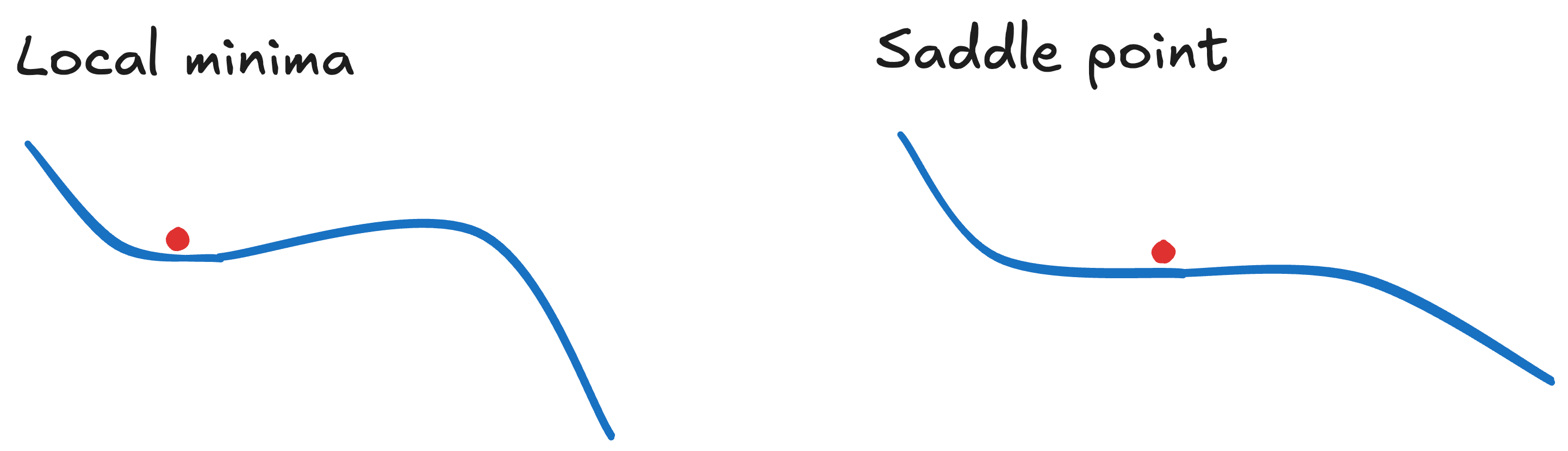
Momentum and Acceleration
To improve SGD’s performance — particularly its zig-zagging in poorly conditioned loss landscapes and getting stuck due to saddle points and local minima — we can add momentum, which smooths updates over time by accumulating gradients.
SGD+Momentum
Core idea: Instead of moving directly in the direction of the current gradient, we use a running sum of gradients (like velocity in physics) to smooth updates. Often scale \(\rho\) is applied.
\(v_{t+1} = \rho v_t + \nabla f(w_t)\)
\(w_{t+1} = w_t - \alpha v_{t+1}\)
Python-style pseudocode:
velocity = 0
while cond is True:
    batch = sample_batch(data)
    weights_grad = evaluate_gradient(loss_func, batch, weights)
    velocity = rho * velocity + weights_grad
    update = velocity
    weights -= learning_rate * update
Typically $\text{rho}$ is between $0.9$ and $0.99$.
Benefits:
- Reduces zig-zagging in poorly conditioned settings.
- Helps escape local minima and saddle points using accumulated velocity.
- Averages out noise from stochastic gradients.
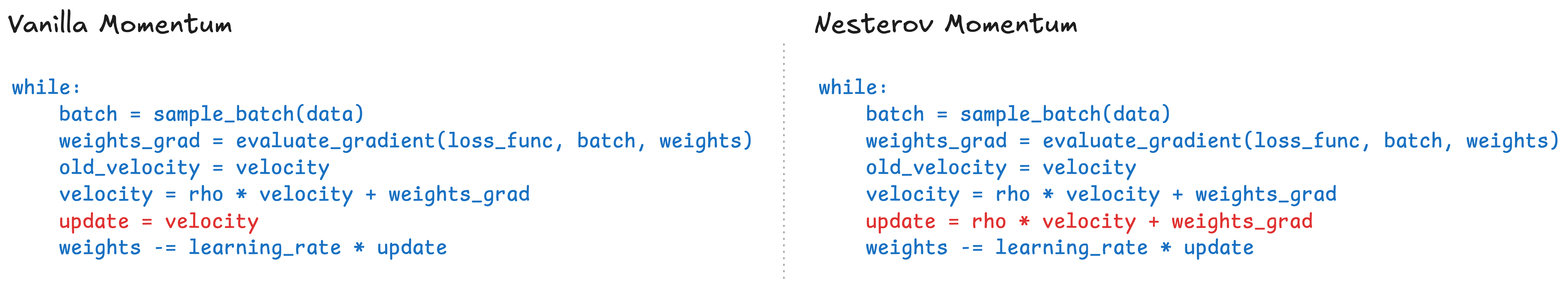
Nesterov Momentum
Core idea: Instead of applying the gradient at the current location, we “look ahead” in the direction of the accumulated momentum:
\(v_{t+1} = \rho v_t - \alpha \nabla f(w_t + \rho v_t)\)
\(w_{t+1} = w_t + v_{t+1}\)
Step 1 - Apply Gradient at the Same Point
To align with vanilla momentum (which computes gradient at \(w_t\)), we can replace \(\hat{w}_t := w_t + \rho v_t\).
Then \(v_{t+1} = \rho v_t - \alpha \nabla f(\hat{w}_t)\).
After rewriting the update in terms of \(\hat{w}_t\): \(w_{t+1} = w_t + v_{t+1} = \hat{w}_t - \rho v_t + v_{t+1}\).
So, \(\hat{w}_{t+1} = w_{t+1} + \rho v_{t+1} = (\hat{w}_t -\rho v_t + v_{t+1}) + \rho v_{t+1}\).
Which finally gives \(\textcolor{blue}{\hat{w}_{t+1} = \hat{w}_t + v_{t+1} + \rho (v_{t+1} - v_t)}\).
Instead of just adding velocity, we add a correction term \(\rho(v_{t+1} - v_t)\).
Step 2 - Make it look closer to Vanilla Momentum
To connect it with a standard momentum form, we define: \(\hat{v}_t := - \frac{v_t}{\alpha} \Leftrightarrow v_t = - \alpha \hat{v}_t\).
Scaling the update: \(v_{t+1} = \rho v_t - \alpha \nabla f(\hat{w}_t) \Leftrightarrow -\frac{v_{t+1}}{\alpha} = \rho (-\frac{v_t}{\alpha}) + \nabla f(\hat{w}_t)\)
So the velocity update becomes like in a standard momentum: \(\textcolor{blue}{\hat{v}_{t+1} = \rho \hat{v}_t + \nabla f(\hat{w}_t)}\).
Now note: \(v_{t+1} - \rho v_t = -\alpha \nabla f(\hat{w}_t)\).
Which gives: \(\hat{w}_{t+1} = \hat{w}_t + v_{t+1} + \rho (v_{t+1} - v_t) = \hat{w}_t + (v_{t+1} -\rho v_t) +\rho v_{t+1} = \hat{w}_t -\alpha \nabla f(\hat{w}_t) - \alpha \rho \hat{v}_{t+1}\).
So we arrive at a familiar-looking update: \(\textcolor{blue}{\hat{w}_{t+1} = \hat{w}_t - \alpha (\nabla f(\hat{w_t}) + \rho \hat{v_{t+1}})}\).
This mirrors vanilla momentum, but with a slightly modified update step:
Python-style pseudocode:
velocity = 0
while cond:
    batch = sample_batch(data)
    weights_grad = evaluate_gradient(loss_func, batch, weights)
    old_velocity = velocity
    velocity = rho * velocity + weights_grad
    update = rho * velocity + weights_grad
    weights -= learning_rate * update
Nesterov momentum provides a slight performance boost over classical momentum by “looking ahead” - this can improve stability and convergence, especially when gradients tend to overshoot minima.
Accumulating Squared Gradients: AdaGrad and RMSProp
Gradient-based optimization can suffer from inconsistent step sizes across dimensions — especially under poor conditioning.
A powerful solution is to adapt the step size per parameter, using accumulated squared gradients to normalize the updates.
AdaGrad
Core idea: Scale down learning rates for parameters that receive large gradients over time. Proposed by John Duchi et al., AdaGrad accumulates the sum of squared gradients and divides each gradient update by the square root of this sum.
\(\text{sq_grad}_{t+1} = \text{sq_grad}_t + (\nabla f(x))^2\)
\(w_{t+1} = w_t - \alpha \frac{\nabla f(x)}{\text{sq_grad}_{t+1} + \epsilon}\)
Python-style pseudocode:
grad_squared_sum = 0
while cond:
    batch = sample_batch(data)
    weights_grad = evaluate_gradient(loss_func, batch, weights)
    grad_squared_sum += weights_grad ** 2
    weights -= learning_rate * weights_grad / (grad_squared_sum ** 0.5 + 1e-7)
It naturally adjusts learning rate based on historical gradient magnitude, and helps to balance poor conditioning. However, there is a problem with Adagrad: step size eventually shrinks to nearly zero due to the growing sum of squared gradients over time.
RMSProp
Core idea: Improve on AdaGrad by introducing a decaying sum of squared gradients - preventing the step size from shrinking too quickly. Originally introduced by Geoff Hinton in his Coursera lectures, it fixes AdaGrad’s issue of vanishing learning rates.
Python-style pseudocode:
grad_squared_sum = 0
while cond:
    batch = sample_batch(data)
    weights_grad = evaluate_gradient(loss_func, batch, weights)
    grad_squared_sum = decay_rate * grad_squared_sum + (1 - decay_rate) * weights_grad ** 2
    weights -= learning_rate * weights_grad / (torch.sqrt(grad_squared_sum) + 1e-7)
Typically, \(\text{decay_rate}\) is \(0.9\) or \(0.99\).
Adam
Core idea: Combine the benefits of momentum and adaptive learning rates into a single optimizer.
Adam (short for Adaptive Moment Estimation) maintains both:
- An exponentially weighted average of past gradients (first moment),
- And an exponentially weighted average of past squared gradients (second moment).
The update rule looks like this:
# Naive Version
first_moment = 0
second_moment = 0
while cond:
    batch = sample_batch(data)
    weights_grad = evaluate_gradient(loss_func, batch, weights)
    first_moment = beta1 * first_moment + (1 - beta1) * weights_grad
    second_moment = beta2 * second_moment + (1 - beta2) * weights_grad ** 2
    x -= learning_rate * first_moment / (torch.sqrt(second_moment) + 1e-7)
In the early steps of training, both first_moment and second_moment are close to zero. This leads to biased estimates, and in the case of second_moment, can cause overly large updates due to division by a very small number — not because of gradient magnitude, but simply due to initialization.
To fix this, Adam applies bias correction factors:
first_moment = 0
second_moment = 0
for t in range(1, num_iterations + 1):
    weights_grad = evaluate_gradient(loss_func, data, weights)
    first_moment = beta1 * first_moment + (1 - beta1) * weights_grad
    second_moment = beta2 * second_moment + (1 - beta2) * weights_grad ** 2
    first_unbias = first_moment / (1 - beta1 ** t)
    second_unbias = second_moment / (1 - beta2 ** t)
    x -= learning_rate * first_unbias / torch.sqrt(second_unbias) + 1e-7
Adam used to be a default choice for many problems. Proposed parameters to start with:
beta1 = 0.9
beta2 = 0.99
learning_rate = 1e-3 # or 5e-4
Adam combines the stability of Momentum with adaptive step size from RMSProp, bias correction improves performance early in training. At the same time, it can sometimes oscillate if used without regularization or learning rate scheduling — particularly in later stages of optimization.
AdamW
Core Idea: Decouple weight decay from the gradient-based optimization step.
To understand misconception with Adam (and other adaptative gradient algorithms), we need to recall what is weight decay, \(L_2\) regularization, and why they are not the same thing.
To understand the need for AdamW, we need to revisit two related but different concepts: weight decay and \(L_2\) regularization. They are often treated as equivalent — but that only holds for standard SGD. In adaptive optimizers, they behave differently.
Weight decay
Weight decay was introduced as an explicit update rule that shrinks the weights at each step (Hanson & Pratt (1988)):
This directly subtracts a portion of the weights themselves on every step — independent of the loss gradient.
L2 regularization
\(L_2\) regularization is applied by modifying the loss function to penalize large weights:
When we take the gradient of this new loss, we get:
\[\nabla f_{L_2}(\theta) = \nabla f(\theta) + \textcolor{red}{2\lambda \theta}\]At first glance, this looks similar to weight decay. And for SGD, it is — they’re equivalent up to scale. But this equivalence breaks down in adaptive optimizers like Adam.
Why This Breaks in Adam
In Adam, gradients are scaled by second-moment estimates (running average of squared gradients). If we add the \(L_2\) term into the gradient, it becomes part of the adaptive scaling. This causes distortions:
Then:
\[g_{t+1}^2 \leftarrow \nabla f(\theta_t)^2 + 4\lambda \nabla f(\theta_t) \theta_t + 4\lambda^2 \theta_t^2\]This means that the regularization term entangles with the loss gradient and gets adaptively rescaled — which is not what we want for weight decay.
AdamW Fix
The AdamW paper proposes to remove the L2 term entirely from the loss and instead apply weight decay outside the gradient calculation:
- No L2 term in the loss. Gradients come only from the task loss.
- Only apply weight decay in the update step:
\(w_{t+1} = w_t - \alpha \left( \frac{\hat{m}_t}{\sqrt{\hat{v}_t} + \epsilon} + 2\textcolor{green}{\lambda w_t} \right)\)
This subtle change restores the correct role of weight decay — shrinking weights uniformly, regardless of the optimizer’s adaptive scaling. As a result, AdamW became the default choice for training large models across NLP and vision.
Beyond Adam: Efficient and Scalable Optimizers
So far, we’ve looked at two major optimizer families: momentum-based and adaptive gradient methods. In this section, I’ll briefly cover four lesser-known optimizers that have shown strong results in practice — especially in large-scale or resource-constrained settings.
AdaFactor
Core Idea: AdaFactor is a memory-efficient optimizer that removes the first moment and approximates the second moment using row- and column-wise averages instead of the full matrix. This reduces memory from \(O(n^2)\) to \(O(n)\) for large matrices, making AdaFactor a practical choice for large models — and it was used to train the T5 language model at scale.
The update rule in python-like pseudo-code is below:
rows_momentum = 0
cols_momentum = 0
beta = 0.9
eps = 1e-30
for t in range(1, num_iterations + 1):
    batch = sample_batch(data)
    weights_grad = evaluate_gradient(loss_func, batch, weights)
    rows_momentum = beta * rows_momentum + (1 - beta) * mean(weights_grad ** 2, axis = 1)
    cols_momentum = beta * cols_momentum + (1 - beta) * mean(weights_grad ** 2, axis = 0)
    x -= learning_rate * weights_grad / torch.sqrt(rows_momentum @ cols_momentum + eps)
Comment: Assumes 2D weight shapes. Works extremely well in practice with minimal memory overhead.
Adan
Core Idea: Adan extends Adam by incorporating a gradient difference term — capturing how the gradient changes over time. Based on the paper, this improves convergence, especially during early training, and helps escape flat regions or noise.
The update rule in python-like pseudocode:
m, v, n = 0, 0, 0
for t in range(1, num_iterations + 1):
    batch = sample_batch(data)
    weights_grad = evaluate_gradient(loss_func, batch, weights)
    delta_g = weights_grad - weights_grad_prev # key difference with Adam / AdamW
    m = beta1 * m + (1 - beta1) * weights_grad
    v = beta2 * v + (1 - beta2) * delta_g
    n = beta3 * n + (1 - beta3) * (g + beta2 * delta_g) ** 2
    # unbias parameters
    m_t, v_t, n_t = m / (1 - beta1**t), v / (1 - beta2**t), n / (1 - beta3**t)
    # make the update
    step_size = lr / (sqrt(n) + eps)
    x -= step_size * (m + beta2 * v)
    # decoupled weight decay
    x /= (1 + weight_decay * lr)
Comment: Following the \(\href{https://arxiv.org/pdf/2208.06677}{\text{paper}}\), it surpasses other optimizers on many backbones and frameworks including ResNet, Transformer-XL, BERT etc.
Lion
Core Idea: \(\href{https://arxiv.org/abs/2302.06675}{\text{Lion}}\) by Chen et al. replaces adaptive scaling with a simpler trick: it uses the sign of the momentum for updates. This significantly reduces computation and memory, while preserving strong convergence - especially in Vision and LLM pretraining.
The update rule in python-like pseudocode is below:
momentum = 0
for t in range(1, num_iterations + 1):
    batch = sample_batch(data)
    weights_grad = evaluate_gradient(loss_func, batch, weights)
    momentum = beta * momentum + (1 - beta) * weights_grad
    x -= learning_rate * torch.sign(momentum)
Comment: Lion is notable for being AI-discovered (via Symbolic Discovery) — a step toward optimizer discovery by AI itself. Note: In my LLM training experiments on TinyStories, Lion consistently achieved the lowest validation cross-entropy loss (~1.4 vs. ~1.5) compared to AdamW and Adan.
Lars and Lamb
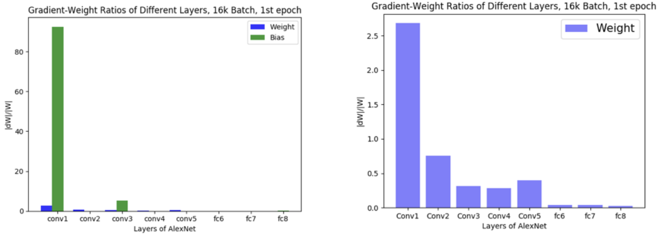
Core Idea: How can we fully leverage supercomputers for deep learning? As hardware scales, training with very large batch sizes becomes attractive due to data parallelism. However, this introduces generalization issues.
It often leads to sharp minima and degraded validation performance (\(\href{https://arxiv.org/pdf/1609.04836}{\text{Keskar et al.}}\), 2017). One key observation is that the ratio between the weight norm and the gradient norm varies significantly across layers (\(\href{https://arxiv.org/pdf/1708.03888v1}{\text{You et al.}}\), 2017), which can destabilize updates. The figure below (from You’s original \(\href{https://pdfs.semanticscholar.org/8905/0de926fc394c941e09b132d86f9f1eab55a2.pdf}{\text{slides}}\)) illustrates how layers has a very different weight-to-gradient norm ratio.
To address this, LARS (Layer-wise Adaptive Rate Scaling) introduces a trust ratio - a scaling factor applied per layer:
\[\text{trust ratio} = \frac{||w||}{||\nabla w|| + \epsilon}\]Later, LAMB (Layer-wise Adaptive Moments for Batch training) extended this idea to adaptive optimizers like Adam, allowing large batch training for Transformers and models like BERT.
Comment: The authors note that:
- SGD + Momentum works well for vision tasks
- Adam / AdamW works well for language tasks
- LARS / LAMB work consistently well across both modalities
In other words: LARS/LAMB unlock large-scale training on supercomputers without sacrificing stability or performance.
Practical Tricks
In practice, optimizer choice is only part of the equation — details like learning rate scheduling, weight decay, and gradient clipping can make or break your training run.
1. Learning Rate Scheduling
A fixed learning rate rarely works throughout training. Most setups use a schedule — like cosine decay, step, or exponential — to start with a higher LR and gradually reduce it for better convergence. Warmup is often used in the first few hundred steps to avoid instability, linearly ramping up the LR before applying the main schedule.
2. Weight Decay vs. L2 Regularization
As discussed in the AdamW section, there’s a common misconception that L2 regularization and weight decay are the same. While both aim to stabilize training by penalizing large weights, they interact differently with adaptive optimizers like Adam.
In short:
- L2 regularization adds a term to the loss and affects gradient calculation.
- Weight decay directly modifies weights during the update step.
3. Gradient Clipping
Sometimes, gradients can explode and destabilize training — especially in RNNs or poorly conditioned loss landscapes. To prevent this, we apply gradient clipping: if the gradient norm exceeds a threshold, we scale it down to a fixed maximum.
4. Batch size and scaling
As discussed in the LARS/LAMB section, modern multi-GPU and TPU setups often use larger batch sizes to fully utilize hardware and accelerate training. However, this introduces two common challenges:
- Optimization instability, especially during early training
- Reduced generalization, as larger batches may converge to sharper minima
Larger batches reduce gradient noise, enabling the use of higher learning rates — but it must be scaled appropriately with batch size (typically linear or square root scaling).
5. Track optimizer metrics
Monitoring optimizer behavior is essential for debugging and tuning:
- Is the gradient norm vanishing?
- Are learning rates behaving as expected?
- Are momentum terms exploding?
Tracking metrics like grad_norm, lr, and other helps catch problems early. Tools like Weights & Biases, TensorBoard, or custom logs can help here.
Beyond the optimizer’s internal logic, training quality is also affected by system-level factors such as mixed precision, numerical stability (e.g., NaNs or overflows), and proper device placement for data and models throughout all training. While these don’t directly alter the optimizer’s behavior, they can lead to silent failures or degraded convergence if not handled carefully.
FLOPs and Optimizer Efficiency
The memory cost of optimizer states can match or exceed that of the model itself — especially with adaptive optimizers — and becomes a major factor in training efficiency, especially for large models.
Here’s a comparison of memory overhead per parameter (for optimizer states):
| Optimizer | Memory Overhead (relative to model size) | Notes |
|---|---|---|
| SGD | \(0\) | No state — just raw weights |
| SGD + Momentum | \(\text{1×}\) | Stores velocity vector |
| Lion | \(\text{1×}\) | Only momentum, no second moment |
| Adam/AdamW | \(\text{2×}\) | First and second moment (m, v) |
| Adan | \(\text{3×}\) | m, v, and gradient diff (n) |
| AdaFactor | \(\sqrt{n}\) | Matrix factorization: row/col means only |
Note: Memory overheads are per parameter unless noted. For AdaFactor, \(\sqrt{n}\) reflects use of row/column averages (for 2D matrices, where n is number of parameters).
These extra states can significantly increase memory consumption and impact training speed and scalability - especially on memory-constrained hardware like GPUs and TPUs.
Conclusion
Gradient-based optimizers remain the main approach in deep learning training. In this post, I explored their evolution — from SGD and Momentum to adaptive variants like Adam and scalable alternatives like LAMB.
Summary Table – Optimizer Trade-offs
| Optimizer | Momentum | Adaptive LR | Memory Overhead | Notes |
|---|---|---|---|---|
| SGD | ❌ | ❌ | \(0\) | No state — just raw weights |
| SGD + Momentum | ✅ | ❌ | \(\text{1×}\) | Stores velocity (1st moment) |
| AdaGrad | ❌ | ✅ | \(\text{1×}\) | Accumulates squared gradients — step size shrinks over time |
| RMSProp | ❌ | ✅ | \(\text{1×}\) | Exponentially decayed average of squared gradients |
| Adam | ✅ | ✅ | \(\text{2×}\) | Maintains m (1st momentum) and v (squared momentum) |
| AdamW | ✅ | ✅ | \(\text{2×}\) | Adam + decoupled weight decay |
| AdaFactor | ❌ | ✅ | \(\sqrt{n}\) | Approximates second moment with row/col averages (2D only) |
| Adan | ✅ | ✅ | \(\text{3×}\) | Adam + gradient difference term: (m, v, n) |
| Lars | ✅ | ❌ | \(\text{1×}\) | Layer-wise “trust ratio” scaling — no adaptive moment history |
| Lamb | ✅ | ✅ | \(\text{2×}\) | AdamW + “trust ratio” — better generalization at large batch sizes |
| Lion | ✅ | ❌ | \(\text{1×}\) | Simple update: sign of momentum, no second moment |
Note: Memory overheads are per parameter unless noted. For AdaFactor, \(\sqrt{n}\) reflects use of row/column averages (for 2D matrices, where n is number of parameters).
Directions That Intrigue Me
One interesting idea is to treat the learning rate as a parameter, rather than a fixed value or manually scheduled hyperparameter. This approach falls under the umbrella of meta-optimization or learning-to-learn. Lion discovered via symbolic program search, reflects a growing interest in searching for optimizers rather than hand-designing them. Earlier, Andrychowicz et al (2016) explored framing optimization itself as a learning problem.
Despite its potential, this area remains niche - and I’m genuinely curious why it hasn’t gained wider traction. Is it instability? Complexity? Or just lack of practical wins (so far)?
Implementation Note
Most discussed above — including Adam, Lion, Adan, and more — are implemented from scratch in my GitHub repo and tested on LLM training on TinyStories.
Enjoy Reading This Article?
Here are some more articles you might like to read next: